It’s Proly like Poly but better

Abstract

Every mathematician I talk to agrees that Poly is an incredibly rich category. How could they not: it’s complete, cocomplete, three orthogonal factorization systems, two monoidal closed structures, its comonoids are categories, etc. And yet there is a common complaint about it, when it comes to modeling. Namely: it’s somehow very discrete, very anchored to Set. Luckily, it looks like the days of disappointing discreteness are behind us. I now think I’ve spent the last 2.5 years enamored by a pale reflection of “the real Poly”, namely what Brandon and I have been calling Proly. I’ll tell you all about it below.

1 Introduction

Every mathematician I talk to agrees that \mathbf{Poly} is an incredibly rich category. How could they not: it’s complete, cocomplete, three orthogonal factorization systems, two monoidal closed structures, its comonoids are categories, etc. And yet there is a common complaint about it, when it comes to modeling. Namely: it’s somehow very discrete, very anchored to \mathbf{Set}.

I was so enamored with \mathbf{Poly}, that I refused to acknowledge these as serious defects, assuming that whatever was missing or wrong would inevitably be ironed out, because something about \mathbf{Poly} is clearly very right. I would say “well, you can consider \mathbf{Poly}_{\mathcal{E}} for any topos \mathcal{E}, so just pick your favorite topos, e.g. the topological topos, and work there”. But on some level it felt hacky; I wanted to have a single category in which to do this sort of work and was disappointed that the object of my mathematical admiration wasn’t enough for people who’s aesthetic sense I appreciated. I had a sense that \mathbf{Poly} should be able to do for applied category theory (ACT) what category theory had done for math—e.g. unify terminology, generalize results, and compress ideas for a large swath of it—but that this destiny was constantly blocked by the unavoidable discreteness at its core.

Luckily, it looks like the days of disappointing discreteness are behind us. I now think I’ve spent the last 2.5 years enamored by a pale reflection of “the real \mathbf{Poly}”, namely what Brandon and I have been calling \mathbf{Proly}.¹ I’ll tell you all about it below. To be clear, even though I’m just getting to understand it now, this is not a new idea: it is well-known that Conduché functors are the exponentiable maps in \mathbf{Cat}, and in Polynomials in Categories with Pullbacks, Mark Weber tells us that you can therefore do polynomial functor stuff with them.² In particular, he showed in Operads as polynomial 2-monads that Cartesian monads in \mathbf{Proly} generalize all sorts of different categorical operad-like structures, including symmetric operads, clubs, etc.

Just like polynomials can be considered as endofunctors on \mathbf{Set} or as combinatorial data from which to build Moore machines, wiring diagrams, cellular automata, think about entropy, etc., prolynomials can be not only be considered as endofunctors on \mathbf{Cat} but also as fascinating presentations of rich combinatorial data. It’s useful to switch back and forth between these perspectives.

Anyway, I claim that \mathbf{Proly} is worth taking a serious look at. What’s so worthwhile about it? First, it has many if not all of the same operations as \mathbf{Poly}: \textsf{0},+,\textnormal{\textsf{1}},\times,\otimes,\mathbin{\triangleleft}, and preliminary work suggests that it’s going to have closures and coclosures, etc., just like \mathbf{Poly}. Second, there is an object \mathfrak{s} in \mathbf{Proly} that acts as a coproduct completion, i.e. \mathfrak{s}\mathbin{\triangleleft}C is the coproduct completion of C, and \mathfrak{s}^\textnormal{op} acts as a product completion, so \mathbf{Poly}=\mathfrak{s}\mathbin{\triangleleft}\mathfrak{s}^\textnormal{op}\mathbin{\triangleleft}\textnormal{\textsf{1}}. In other words, \mathbf{Poly} is not only a full subcategory of \mathbf{Proly}, it’s also an object.³ Third, comonoids in \mathbf{Proly} are double categories, pseudocomonoids are pseudo-double categories, and coalgebras simultaneously generalize copresheaves and actegories. I’ll explain all this, albeit pretty briefly, below.

I’ve benefited greatly from conversations with Brandon Shapiro. Indeed, I had been thinking of many of the ideas below in terms of functors \mathcal{C}\to\mathbf{Cat}, and only during a conversation with Brandon did we realize that it’s much better to use functors \mathcal{C}\to\mathbf{Prof}, a crucial insight. Thanks to Nate Soares who caught an error that we were making.⁴ A lot of the background ideas germinated also in talking with Josh Meyers, who is a research associate at Topos this summer. I’ve also benefited from conversations with David Jaz Myers and David Dalrymple.

None of the following has been formally proven, so take the claims with a grain of salt. In particular, all errors are my own.

2 What is \mathbf{Proly}?

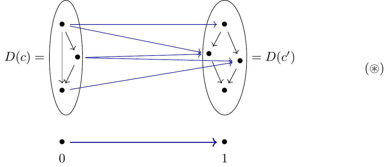
An object in \mathbf{Proly} is a pair (C,D), where C is a category and D\colon C\to\mathbf{Prof} is a normal pseudofunctor to the bicategory \mathbf{Prof} of categories and profunctors.⁵ This may sound difficult, but the first thing to recognize is that the objects in \mathbf{Prof} are categories, so for every object c\in C, we have a category D(c)\in\mathbf{Cat}. For every morphism f\colon c\to c' in C, we have a profunctor D(f)\colon D(c)\nrightarrow D(c'), i.e. a functor D(c)^\textnormal{op}\times D(c')\to\mathbf{Set}. I often think of this in terms of its collage, which you can imagine like a bordism, or category-with-boundary, as shown here:

This suggests another way to look at an object in \mathbf{Proly}, namely as something called a Conduché fibration. In other words, you can take the Grothendieck construction of D and get a category \int D, equipped with a functor P\colon\int D\to C, at which point we’d see (\circledast) as what’s happening over a single morphism in C. That is, above every object downstairs in C is a whole category D(c), and above every morphism in C is a bordism, i.e. the collage of a profunctor as shown in (\circledast). The functor P has the further property that maps upstairs who can be factored downstairs can also be factored upstairs. A more precise definition of Conduché fibration is given on the nLab.

As usual, it’s important to consider the morphisms between these Conduché fibrations: we want the polynomial ones. A map (C_1,D_1)\to(C_2,D_2) consists of a pair of functors (\varphi,\varphi^\sharp) of the form

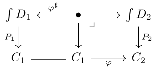
i.e. a functor \varphi\colon C_1\to C_2 and a functor \varphi^\sharp\colon (C_1\times_{C_2}\int D_2)\to D_1 from the pullback to D_1. Note that if you restrict every category here to be discrete, you get back \mathbf{Poly}.

What it means that Conduché functors Q\colon E\to B are (precisely the) exponentiable maps in \mathbf{Cat} is that the pullback functor Q^*\colon\mathbf{Cat}/B\to\mathbf{Cat}/E has a right adjoint, denoted \prod_Q. For any functor Q, the pullback Q^* has a left adjoint, denoted \sum_Q. What’s really great is that these two things always distribute (thanks Mark Weber!). So we can use the usual polynomial notation for prolynomials: q\coloneqq\sum_{b\in B}\mathcal{y}^{E[b]}\cong\sum_{b\in B}\prod_{e\in E[b]}\mathcal{y} where E[b]\coloneqq Q^{-1}(b) is the category given by the fiber over b.⁶

Currently I’m thinking of an arbitrary p:\mathbf{Proly} p\colon \sum_{I\in p(1)}\mathcal{y}^{p[I]} as “the p(1)-indexed family of p-shaped categories and bordisms”. Here’s my current preferred terminology for the data involved:

In the display above, I’ve included another pictorial perspective, a 90^\circ rotation and redrawing of (\circledast), which might help later in understanding how to think of comonoids in \mathbf{Proly} as double categories.

Next, I’ll talk about some operations, but it gets a bit technical, and the reader might want to skip ahead to the example section for motivation.

3 Operations

Just like polynomials have \textsf{0},\textnormal{\textsf{1}},+,\times,\mathcal{y},\otimes,\mathbin{\triangleleft} and many other operations, so do prolynomials. I haven’t checked closures and coclosures yet, so let’s stick with what I’m more confident in. The \textsf{0}-prolynomial corresponds to the identity fibration \textsf{0}\to \textsf{0}, and the \textnormal{\textsf{1}}-prolynomial corresponds to \textsf{0}\to \textnormal{\textsf{1}}. The sum of two prolynomials is given by “sum on the top and bottom” (E_1\to B_1)+(E_2\to B_2)=(E_1+E_2)\to (B_1+B_2) and the tensor product is similarly just “product on the top and bottom”: (E_1\to B_1)\otimes(E_2\to B_2)=(E_1\times E_2)\to (B_1\times B_2). Their Cartesian product is (E_1\to B_1)\times(E_2\to B_2)=(E_1\times B_2+E_2\times B_1)\to (B_1\times B_2). In each case, you can also express the new prolynomial in terms of a category with a map to \mathbf{Prof}; e.g. the above product is the map (B_1\times B_2)\to\mathbf{Prof} that sends (b_1,b_2) to the sum E_1[b_1]+E_2[b_2].

The \mathbin{\triangleleft} operation is the most interesting. We could denote it simply using \Sigma’s and \Pi’s as usual: p\mathbin{\triangleleft}q=\sum_{I\in p(\textnormal{\textsf{1}})}\;\prod_{i\in p[I]}\;\sum_{J\in q(\textnormal{\textsf{1}})}\;\prod_{j\in q[J]}\mathcal{y} but, as we said above, you need to interpret \Sigma and \Pi as operations in \mathbf{Cat}. Luckily, the notation can be unpacked. The first thing to do is move the \Pi past the \Sigma. \begin{aligned} p\mathbin{\triangleleft}q&=\sum_{I\in p(\textnormal{\textsf{1}})}\;\sum_{J\colon p[I]\to q(\textnormal{\textsf{1}})}\;\prod_{i\in p[I]}\;\prod_{j\in q[Ji]}\;\mathcal{y}\\&\cong \sum_{I\in p(\textnormal{\textsf{1}})}\;\sum_{J\colon p[I]\to q(\textnormal{\textsf{1}})}\mathcal{y}^{\;\sum\limits_{i\in p[I]}q[Ji]}\end{aligned} It says that the underlying category p\mathbin{\triangleleft}q(\textnormal{\textsf{1}}) of the composite is \sum_{I\in p(\textnormal{\textsf{1}})}\;\sum_{J\colon p[I]\to q(\textnormal{\textsf{1}})}1; what does that mean? It means an object consists of a pair (I,J) where I\in p(\textnormal{\textsf{1}}) is an object and J\colon p[I]\to q(\textnormal{\textsf{1}}) is a functor. A morphism consists of map F\colon I\to I' in p(\textnormal{\textsf{1}}) and a square

Can you see J\colon p[I]\to q(\textnormal{\textsf{1}}) as a p-shaped category in q(\textnormal{\textsf{1}}) and F^\flat\colon p[F]\to q(1) as a p-shaped bordism in q(\textnormal{\textsf{1}})?

Anyway, the notation packs a punch, but in some sense it’s pretty “follow-your-nose” once you get the hang of it. What is the functor \sum_{I\in p(\textnormal{\textsf{1}})}\;\sum_{J\colon p[I]\to q(\textnormal{\textsf{1}})}\to\mathbf{Prof} that has been notated \sum_{i\in p[I]}q[Ji]? Again, you can kinda read it off. Since for each the object (I,J) we have a category p[I] and profunctorially for each i\in p[I] another category q[Ji], one might guess that we’re supposed to add all these q’s up. Indeed, \sum_{i\in p[I]}q[Ji] denotes the corresponding Grothendieck construction.

4 Examples

Fibrations.

Every opfibration and every fibration in \mathbf{Cat} is also a Conduché fibration, because they can be identified with pseudofunctors D\colon C\to\mathbf{Cat} and D\colon C\to\mathbf{Cat}^\textnormal{op}, and we have embeddings \mathbf{Cat}\to\mathbf{Prof}\leftarrow\mathbf{Cat}^\textnormal{op}. Moreover, the opposite P^\textnormal{op}\colon E^\textnormal{op}\to B^\textnormal{op} of any Conduché fibration is also Conduché. So given a map D\colon C\to\mathbf{Cat}, we’d think of it as the C-indexed world of D-shaped categories and functors.

Linears and constants.

For any category C, the identity map C\to C stands in as the associated “linear” prolynomial C\mathcal{y}, and the unique map 0\to C stands in as the “constant” prolynomial C. Morphisms between them in \mathbf{Proly} are just functors.

Polynomials are a full subcategory.

Given any polynomial functor p:\mathbf{Poly}, we can regard p(\textnormal{\textsf{1}}) as a discrete category, and for each I\in p(\textnormal{\textsf{1}}) we can regard p[I] as a discrete category. Because p(\textnormal{\textsf{1}}) has only identity maps, we don’t need to provide any profunctors in order to regard p as a prolynomial. Polynomials thus embed as a full subcategory of prolynomials. They are discretely-indexed worlds of discrete categories and functions.

Coproduct completion.

The inclusion \mathbf{Set}\to\mathbf{Cat}, given by sending a set A to itself as a discrete category, corresponds to the opfibration \mathbf{Set}_*\to\mathbf{Set} sending a pointed set (A,a) to its underlying set A. Let’s denote the corresponding prolynomial by \mathfrak{s}\coloneqq\sum_{A\in\mathbf{Set}}\mathcal{y}^A. This is the \mathbf{Set}-indexed world of discrete categories and functions.

For any category C, the category \mathfrak{s}\mathbin{\triangleleft}C is the coproduct completion of C. Indeed, an object of it consists of a set A and an object c_a\in C for every a\in A. A morphism in it consists of a function f\colon A\to A' and for every a\in A a morphism c_a\to c'_{fa}.

Product completion.

The opposite of \mathfrak{s} is the fibration \mathfrak{s}^\textnormal{op}\coloneqq (\mathbf{Set}_*^\textnormal{op}\to\mathbf{Set}^\textnormal{op}). For any category C, the composite s^\textnormal{op}\mathbin{\triangleleft}C is the product completion of C.

\mathbf{Poly} and \mathbf{Dir}.

We can find the category of (small) polynomial functors as an object in \mathbf{Proly} because it is the free coproduct completion of the free product completion of \textnormal{\textsf{1}}. In other words \mathbf{Poly}=\mathfrak{s}\mathbin{\triangleleft}\mathfrak{s}^\textnormal{op}\mathbin{\triangleleft}\textnormal{\textsf{1}}. Similarly, the category of Dirichlet polynomials is \mathfrak{s}\mathbin{\triangleleft}\mathfrak{s}\mathbin{\triangleleft}\textnormal{\textsf{1}}, the free coproduct completion of the free coproduct completion of \textnormal{\textsf{1}}. The distributive law I was looking for in this blog post was in fact \mathfrak{s}^\textnormal{op}\mathbin{\triangleleft}\mathfrak{s}\to\mathfrak{s}\mathbin{\triangleleft}\mathfrak{s}^\textnormal{op}.

Several of the monoidal products on \mathbf{Poly} (so far, I’ve successfully tried +, \times, \otimes, and \mathbin{\triangleleft}) can be constructed as maps (\mathfrak{s}\mathbin{\triangleleft}\mathfrak{s}^\textnormal{op}\mathbin{\triangleleft}\textnormal{\textsf{1}})\otimes (\mathfrak{s}\mathbin{\triangleleft}\mathfrak{s}^\textnormal{op}\mathbin{\triangleleft}\textnormal{\textsf{1}})\to (\mathfrak{s}\mathbin{\triangleleft}\mathfrak{s}^\textnormal{op}\mathbin{\triangleleft}\textnormal{\textsf{1}}) using simpler structures and properties.⁷

Comonoids are double categories.

Ahman and Uustalu showed that comonoids in \mathbf{Poly} are exactly categories. For any locally cartesian closed category \mathcal{E}, the comonoids in \mathbf{Poly}_{\mathcal{E}}(1,1) are categories internal to \mathcal{E}. A double category is by definition a category internal to \mathbf{Cat}, but since \mathbf{Cat} is not LCC, comonoids in it are double categories with a special property. Similarly, pseudo-comonoids are pseudo-double categories with a certain property.⁸ Given a prolynomial p=\sum_{I\in p(\textnormal{\textsf{1}})}\mathcal{y}^{p[I]} and a comonoid structure (p,\epsilon,\delta), there is a double category \mathbb{P}=\mathbb{P}_1\underset{r}{\overset{l}{\rightrightarrows}}\mathbb{P}_0 whose vertical category is \mathbb{P}_0=p(\textnormal{\textsf{1}}). The associated Conduché fibration is l\colon \mathbb{P}_1\to \mathbb{P}_0, and for each object I\in p(\textnormal{\textsf{1}}), the category p[I] is that of all horizontal maps out of I, i.e. the preimage l^{-1}(I)=p[I]. Given f\colon I\to I' in p(\textnormal{\textsf{1}}), the profunctor p[f]\colon p[I]\nrightarrow p[I'] is that of all 2-cells. And the data of identity, codomain, and composition for horizontal arrows and 2-cells is given by the comonoid structure (\epsilon,\delta).

For example, if \mathcal{C} is a bicategory, then its double category of quintets is carried by the prolynomial \sum_{c\in \mathcal{C}}\mathcal{y}^{c/\!/\mathcal{C}}, where c/\!/\mathcal{C} denotes the lax coslice category. As another example, the pseudodouble category of spans is simply the coclosure \left[\begin{smallmatrix}{\vphantom{f}\mathfrak{s}\mathbin{\triangleleft}\mathfrak{s}} \\ {\vphantom{f}\mathfrak{s}} \end{smallmatrix}\right], which carries a pseudocomonoid structure for formal reasons, since \mathfrak{s} carries a (pseudo)monoid structure.

Delta lenses.

For any category C, consider the coslice functor C\to\mathbf{Cat}^\textnormal{op}\subseteq\mathbf{Prof} given by c\mapsto c/C \qquad\text{and}\qquad (c\xrightarrow{f} c')\mapsto \big(c/C\xleftarrow{g\mapsto (f\mathbin{;}g)}c'/C\big) This prolynomial would be denoted \Delta_C\coloneqq\sum_{c\in C}\mathcal{y}^{c/C}. It’s a special case of the quintet construction above, and hence comes with a comonoid structure that identifies it with the double category of commutative squares in C. A \mathbf{Proly}-comonoid map from \Delta_C\to\Delta_D is the same as a Delta-lens from C to D in the sense of Diskin.

Monoidal categories.

A set M carries a monoid structure in \mathbf{Set} iff the polynomial \mathcal{y}^M carries a comonoid structure in \mathbf{Poly}. Similarly, a category M carries a monoidal structure (is a pseudomonoid in \mathbf{Cat}) iff \mathcal{y}^M carries a pseudocomonoid structure in \mathbf{Proly}. This makes \mathcal{y}^M a vertically-trivial pseudodouble category, i.e. a bicategory with one object, as expected.

Coalgebras generalize copresheaves and actegories.

In \mathbf{Poly}, a coalgebra A\to c(A) for a comonoid c is copresheaf, or technically a discrete opfibration into the category c. In \mathbf{Proly}, a comonoid is a double category, so what is a coalgebra there? I still haven’t really understood it, but when the carrier of c comes from the full subcategory of polynomials, the corresponding double category is vertically discrete and has no 2-cells, and the coalgebra is just a copresheaf as before. The only other case I really understand well is when c=\mathcal{y}^M is a monoidal category, in which case a \mathcal{y}^M-coalgebra is an actegory, i.e. a category A and an action M\times A\to A.

5 Conclusion

I’m quite enamored with prolynomials. I don’t exactly feel like it’s a “new love” because as we saw above, \mathbf{Poly} embeds fully faithfully into \mathbf{Proly}, and if things go as I expect, prolynomials should have many if not all of the same monoidal and closure operations as polynomials. It will be interesting to explore what they all mean, what cofunctors and bicomodules tell us, etc. And hopefully, we’ll find real-life applications, i.e. more robust ways to think about information, communication, interaction, etc. in this language.

I’ll close with some workfun for the interested reader.

6 Workfun for the interested reader

• Open contemplation… What might motivate a person with less background knowledge of category theory to learn more about the subject of this blogpost?

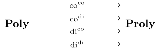
• Vocabulary… Considering that every set can be made into a discrete category and a codiscrete category, Define functors with the following names:

  

• Exercise… Do any of the above functors have adjoints? Concisely explain your process in thinking about this.

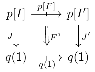
• Challenge… Define lens-coclosure \left[\begin{smallmatrix}{\vphantom{f}-} \\ {\vphantom{f}-} \end{smallmatrix}\right] and multi-coclosure \frown for \mathbf{Proly} as one does in \mathbf{Poly}. Interpret the data of a pair (g,t) where g\in\mathbf{Proly} is a prolynomial and t is an arbitrary map of the form: \dot{p}(1)\mathcal{y}\cong \begin{bmatrix}{\vphantom{f_f^f}1} \\ {\vphantom{f_f^f}p(1)\overset{\mathrm{id}}{\frown} p} \end{bmatrix} \xrightarrow{\;\;t\;\;} p

Footnotes

1. Out of all the names one might choose for this category this one is proly the most fun one to say. The only other justification for the name \mathbf{Proly} is that it involves profunctors. But the name very well may change, or \mathbf{Proly} may end up just being our pet name for something more canonical.

2. Here, we’re focusing on what Weber would call \mathbf{Proly}\coloneqq\mathbf{Poly}_{\mathbf{Cat}}(\textnormal{\textsf{1}},\textnormal{\textsf{1}}). I imagine that, just like (\mathbf{Poly},\mathcal{y},\mathbin{\triangleleft}) is only the monoidal category of polynomials in one variable, and yet its framed bicategory of comonoids subsumes the usual bicategory of polynomials in many variables, we may find that we can find that comonoids in \mathbf{Proly}=\mathbf{Poly}_{\mathbf{Cat}}(\textnormal{\textsf{1}},\textnormal{\textsf{1}}) in fact subsumes the rest of Weber’s \mathbf{Poly}_{\mathbf{Cat}}. But this remains to be seen.

3. Throughout this post I’ll be a bit fast and loose with size issues. For example, here I should really fix a universe and talk about large polynomials and small polynomials, etc.

4. While comonoids in \mathbf{Proly} are double categories, I was under the impression that the converse was also true. However, Nate helped us realize that not all double categories are comonoids in \mathbf{Proly}, basically because \mathbf{Cat} is not locally cartesian closed.

5. That D is a normal pseudofunctor means that identities in C are sent to identity profunctors and that there is an isomorphism D(f)\mathbin{;}D(g)\cong D(f\mathbin{;}g), rather than an equality.

6. Once one defines the substitution product \mathbin{\triangleleft}, it is easy to check that there is an isomorphism of categories p(\textnormal{\textsf{1}})\cong B.

7. For example, to get +, you use that for any p,q\in\mathbf{Proly}, there is an isomorphism (p\otimes q)\mathbin{\triangleleft}1\cong(p\times q)\mathbin{\triangleleft}1. Then (\mathfrak{s}\mathbin{\triangleleft}\mathfrak{s}^\textnormal{op}\mathbin{\triangleleft}\textnormal{\textsf{1}})\otimes (\mathfrak{s}\mathbin{\triangleleft}\mathfrak{s}^\textnormal{op}\mathbin{\triangleleft}\textnormal{\textsf{1}})\cong(\mathfrak{s}\mathbin{\triangleleft}\mathfrak{s}^\textnormal{op}\mathbin{\triangleleft}\textnormal{\textsf{1}})\times(\mathfrak{s}\mathbin{\triangleleft}\mathfrak{s}^\textnormal{op}\mathbin{\triangleleft}\textnormal{\textsf{1}})\cong(\mathfrak{s}\times\mathfrak{s})\mathbin{\triangleleft}(\mathfrak{s}^\textnormal{op}\mathbin{\triangleleft}1). There is a map \mathfrak{s}\times\mathfrak{s}\to\mathfrak{s} sending S,T to the coproduct S+T, and thus we obtain the desired map (\mathfrak{s}\mathbin{\triangleleft}\mathfrak{s}^\textnormal{op}\mathbin{\triangleleft}\textnormal{\textsf{1}})\otimes (\mathfrak{s}\mathbin{\triangleleft}\mathfrak{s}^\textnormal{op}\mathbin{\triangleleft}\textnormal{\textsf{1}})\to(\mathfrak{s}\mathbin{\triangleleft}\mathfrak{s}^\textnormal{op}\mathbin{\triangleleft}\textnormal{\textsf{1}}).

8. The property is that the source map s\colon\mathbb{D}_1\to\mathbb{D}_0 is Conduche. Every proarrow equipment satisfies this property, though it’s much more general.