Decorated cospans via the Grothendieck construction

Abstract

Building on the double Grothendieck construction introduced last time, we explain how decorated cospans are instance of the Grothendieck construction. This perspective suggests a natural generalization of decorated cospans, which we illustrate through several examples.

Decorated cospans turn closed systems into open ones, which can be composed along their boundaries to form larger systems (Fong 2015). Continuous dynamical systems and a variety of combinatorial systems, such as graphs, Petri nets, and stock and flow diagrams, have all been made into open systems using this method. In addition, decorated cospans are thought to be more general than their simpler cousin, structured cospans (Baez, Courser, and Vasilakopoulou 2022).

Despite this versatility, decorated cospans do not encompass all categories with morphisms that could reasonably be called “cospans with decorations.” The standard example of decorated cospans are open graphs, made open by exposing vertices via a cospan of vertex sets. Yet the other kind of open graphs—those allowing “dangling edges,” where the incoming edges define the domain and the outgoing edges the codomain—are not decorated cospans, even though they can also be described as cospans, now of edge sets, plus some extra data. We know that because decorated cospan categories are “undirected” (more accurately, they are hypergraph categories), whereas the category of graphs with dangling edges has a definite directionality. In this post, we’ll explain how to generalize decorated cospans to include this and other interesting examples.

To do that, we’ll use the Grothendieck construction for double categories introduced in our previous blog post. It would be helpful to read that post before this one, but it’s not strictly necessary since we’ll review the specific case of the construction that we need. We’ll also start with a brief review of decorated cospans. For much more about decorated cospans, see the papers cited above or the several blog posts written over the years by John Baez at the n-Category Cafe.

Update (03 April 2023): I have incorporated the content of this blog post into a new paper (Patterson 2023).

1 Review of decorated cospans

Given a category $\mathsf{A}$ with finite colimits and a lax monoidal functor $F: (\mathsf{A},+) \to (\mathsf{Set},\times)$, the category of $F$-decorated cospans has:

• objects, the objects of $\mathsf{A}$;
• morphisms $a \to b$, isomorphism classes of a cospan $a \rightarrow m \leftarrow b$ in $\mathsf{A}$ together with an element $s \in F(m)$.

For example, to obtain the category of isomorphism classes of open graphs, made open along vertices, we take the lax monoidal functor $F: (\mathsf{FinSet}, +) \to (\mathsf{Set},\times)$ that sends a finite set $V$ to the set $F(V)$ of graphs with vertex set $V$. Its laxators $$F(U) \times F(V) \to F(U+V), \qquad U,V \in \mathsf{FinSet}$$ send a pair of graphs $G$ and $H$ having vertex sets $U$ and $V$ to the coproduct graph $G+H$ with vertex set $U+V$.

The original version of decorated cospans forgets about any morphisms which may have already existed between the original (closed) systems. In the case of open graphs, these morphisms are graph homomorphisms. Their absence is often a problem! To recover them, we need a more refined version of decorated cospans, furnishing not just a category but a double category.

Given a category $\mathsf{A}$ with finite colimits and a lax monoidal functor $F: (\mathsf{A},+) \to (\mathsf{Cat},\times)$, the double category of $F$-decorated cospans has:

• objects, the objects of $\mathsf{A}$;
• arrows, the morphisms of $\mathsf{A}$;
• proarrows $a \to b$, a cospan $a \rightarrow m \leftarrow b$ in $\mathsf{A}$ together with an object $s \in F(m)$;
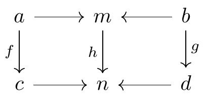
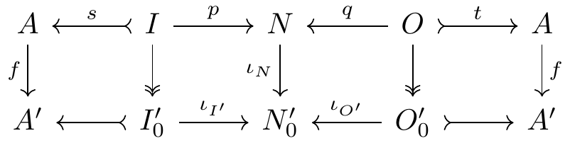
• cells $(a \rightarrow m \leftarrow b, s) \Rightarrow(c \rightarrow n \leftarrow d, t)$, a map of cospans in $\mathsf{A}$, which is a commuatative diagram of the form below, together with a morphism $\nu: F(h)(s) \to t$ in $F(n)$.

To get a double category of open graphs, we take the lax monoidal functor $F: (\mathsf{FinSet}, +) \to (\mathsf{Cat}, \times)$ that sends a finite set $V$ to the category $F(V)$ of graphs with vertex set $V$, whose morphisms are vertex-preserving graph homomorphisms. A cell—or rather the apex part of a cell—from a graph $G$ with vertex set $U$ to a graph $H$ with vertex set $V$ then consists of a function $h: U \to V$ together with a vertex-preserving graph homomorphism $\nu: F(h)(G) \to H$. Together, the two functions $h$ and $\nu$ are equivalent to an arbitrary graph homomorphism $G \to H$, namely the one with vertex map $h$ and edge map $\nu_E$.

2 A modular reconstruction of decorated cospans

Last time, we introduced a Grothendieck construction for double categories, whose input data is a lax double functor $\mathbb{D} \to \mathbb{S}\mathsf{pan}(\mathsf{Cat})$. To decorate cospans, we apply the construction on the (pseudo) double category $\mathbb{D} = \mathbb{C}\mathsf{sp}(\mathsf{A})$ of cospans in a finitely cocomplete category $\mathsf{A}$. In other words, the input data for generalized decorated cospans is a lax double functor $\mathbb{C}\mathsf{sp}(\mathsf{A}) \to \mathbb{S}\mathsf{pan}(\mathsf{Cat})$. We will describe the Grothendieck construction of such a double functor in the next section. First, let’s see how this data generalizes the usual data for decorated cospans, a lax monoidal functor $(\mathsf{A},+) \to (\mathsf{Cat},\times)$. To do that, we’ll use three simple mappings.

Mapping #1. A monoidal category can be seen as a double category $\mathbb{D}$ whose underlying 1-category $\mathbb{D}_0$ is trivial. This fact is a variation on the possibly more familar one that a monoidal category is a bicategory with one object. More precisely, for any monoidal category $(\mathsf{C},\otimes)$, there is a double category $\mathbb{M}(\mathsf{C},\otimes)$ with $\mathbb{M}(\mathsf{C},\otimes)_0 = \mathsf{1}$, the terminal category, and $\mathbb{M}(\mathsf{C},\otimes)_1 = \mathsf{C}$. External composition and identities are given by the monoidal product and unit. A lax monoidal functor can also be viewed as a lax double functor, so altogether we obtain a functor $$\mathbb{M}: \mathsf{MonCat}_{\mathrm{lax}} \to \mathsf{DblCat}_{\mathrm{lax}}.$$

Mapping #2. For any category $\mathsf{A}$ with finite colimits, the apex double functor is the lax double functor $$\operatorname{Apex}: \mathbb{C}\mathsf{sp}(\mathsf{A}) \to \mathbb{M}(\mathsf{A},+)$$ with $\operatorname{Apex}_0: \mathsf{A} \xrightarrow{!} \mathsf{1}$ the unique map and $\operatorname{Apex}_1 := \operatorname{apex}: \mathsf{A}^\mathsf{Csp}\to \mathsf{A}$ the apex functor, where we write $\mathsf{Csp}:= \{\bullet \rightarrow \bullet \leftarrow \bullet\}$ for the walking cospan. For composable cospans $m := (a \rightarrow x \leftarrow b)$ and $n := (b \rightarrow y \leftarrow c)$ in $\mathsf{A}$, the laxators $$\operatorname{Apex}_1(m) + \operatorname{Apex}_1(n) = x + y \xrightarrow{[\iota_x, \iota_y]} x +_b y = \operatorname{Apex}_1(m \odot n),$$ as well as unitors $0 \xrightarrow{!} a$ for $a \in \mathsf{A}$, are given by the universal properties of the colimits.

Mapping #3. For any category $\mathsf{C}$ with finite limits, the codiscrete span functor is the double functor $$\operatorname{coDisc}: \mathbb{M}(\mathsf{C}, \times) \to \mathbb{S}\mathsf{pan}(\mathsf{C})$$ with $\operatorname{coDisc}_0: \mathsf{1} \to \mathsf{C}$ picking out the terminal object $1$ of $\mathsf{C}$ and $\operatorname{coDisc}_1: \mathsf{C} \to \mathsf{C}^\mathsf{Span}$ sending each object $c \in \mathsf{C}$ to the codiscrete span $1 \xleftarrow{!} c \xrightarrow{!} 1$. This double functor is pseudo, and can be made strict by a suitable choice of limits.

It is now clear how the usual data for decorated cospans, a lax monoidal functor $(F, \Phi, \phi): (\mathsf{A},+) \to (\mathsf{Cat},\times)$, gives rise to data for a Grothendieck construction on the double category of cospans in $\mathsf{A}$. We apply the functor $\mathbb{M}: \mathsf{MonCat}_{\mathrm{lax}} \to \mathsf{DblCat}_{\mathrm{lax}}$, then precompose with $\operatorname{Apex}$ and postcompose with $\operatorname{coDisc}$: $$\tilde{F}: \mathbb{C}\mathsf{sp}(\mathsf{A}) \xrightarrow{\operatorname{Apex}} \mathbb{M}(\mathsf{A},+) \xrightarrow{\mathbb{M}(F)} \mathbb{M}(\mathsf{Cat},\times) \xrightarrow{\operatorname{coDisc}} \mathbb{S}\mathsf{pan}(\mathsf{Cat}).$$ The resulting lax double functor $\tilde{F}$ sends each object $a \in \mathsf{A}$ to the trivial category $\mathsf{1}$ and sends a cospan $a \rightarrow m \leftarrow b$ in $\mathsf{A}$ to the span of categories $\mathsf{1} \xleftarrow{!} F(m) \xrightarrow{!} \mathsf{1}$. For composable cospans $m = (a \rightarrow x \leftarrow b)$ and $n = (b \rightarrow y \leftarrow c)$, the laxator $$\tilde F(m) \odot \tilde F(n) \to \tilde F(m \odot n)$$ is the image under $\operatorname{coDisc}$ of the composite $$F(x) \times F(y) \xrightarrow{\Phi_{x,y}} F(x+y) \xrightarrow{F[\iota_x,\iota_y]} F(x +_b y)$$ in $\mathsf{Cat}$. The unitor of $\tilde F$ at the object $a \in \mathsf{A}$ is the image under $\operatorname{coDisc}$ of $$\mathsf{1} \xrightarrow{\phi} F(0) \xrightarrow{F(!)} F(a).$$ The last two formulas are precisely the ones used to compose decorated cospans (Fong 2015), (Baez, Courser, and Vasilakopoulou 2022).

This observation clears up a puzzle that had always slightly bothered me about decorated cospans: where does the composition law come from? Why does it involve two operations, instead of just one? Well, the answer is that the construction itself involves a composite! Specifically, it is precomposition with the lax double functor $\operatorname{Apex}: \mathbb{C}\mathsf{sp}(\mathsf{A}) \to \mathbb{M}(\mathsf{A},+)$ that gives the distinctive composition law for decorated cospans. Using this modular reconstruction of decorated cospans, we can start with various kinds of lax monoidal or double functors, but ultimately reduce them all to data for a Grothendieck construction on the double category of cospans.

3 Double Grothendieck construction on cospans

We now apply the double Grothendieck construction to decorate double categories of cospans. Abstractly speaking, this is no more than taking the Grothendieck construction of a lax double functor $\mathbb{D} \to \mathbb{S}\mathsf{pan}(\mathsf{Cat})$, as defined in the previous blog post, in the particular case that $\mathbb{D}$ is a double category of cospans. For the sake of clarity and concreteness, we are going to spell that out in some detail. Further technical details can found in the previous post.

Let $\mathsf{A}$ be a category with finite colimits and let $(\tilde F, \tilde\Gamma, \tilde\gamma): \mathbb{C}\mathsf{sp}(\mathsf{A}) \to \mathbb{S}\mathsf{pan}(\mathsf{Cat})$ be a lax double functor. Define the two functors $$F_0 := \tilde F_0: \mathsf{A} \to \mathsf{Cat}, \qquad F_1 := \operatorname{apex}\circ \tilde F_1: \mathsf{A}^\mathsf{Csp}\to \mathsf{Cat}$$ and the two natural transformations

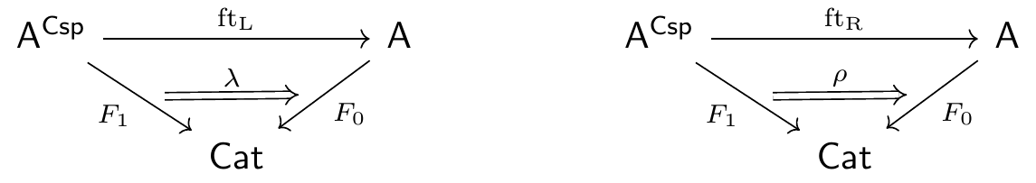
having components $\lambda_m := \operatorname{leg}_L(\tilde F_1(m))$ and $\rho_m := \operatorname{leg}_R(\tilde F_1(m))$, where $\operatorname{leg}_L, \operatorname{leg}_R: \mathsf{Cat}^\mathsf{Span}\to {\mathsf{Cat}}^{\rightarrow}$ extract the left and right legs of a span. The components are well-defined because, since $\tilde F$ is a double functor, $\operatorname{ft}_L(\tilde F_1(m)) = \tilde F_0(\operatorname{ft}_L(m))$ and $\operatorname{ft}_R(\tilde F_1(m)) = \tilde F_0(\operatorname{ft}_R(m))$.

The double category of $F$-decorated cospans is the Grothendieck construction $\int F$, which has underlying categories $(\int F)_0 = \int F_0$ and $(\int F)_1 = \int F_1$. Explicitly, it has:

• objects, pairs $(a,x)$ with an object $a \in \mathsf{A}$ and a decorating object $x \in F_0(a)$;
• arrows $(a,x) \to (b,y)$, pairs $(f,\phi)$ with a morphism $f: a \to b$ in $\mathsf{A}$ and a decoration morphism $\phi: F_0 f(x) \to y$ in $F_0(b)$;
• proarrows, pairs $(m,s)$ with a cospan $m = (a \rightarrow q \leftarrow b)$ in $\mathsf{A}$ and a decorating object $s \in F_1(m)$;
• cells $(m,s) \to (n,t)$, pairs $(\alpha,\nu)$ with a map $\alpha: m \to n$ of cospans in $\mathsf{A}$ and a decoration morphism $\nu: F_1 \alpha(s) \to t$ in $F_1(n)$.

Sources and targets in $\int F$ are defined by the functors $\int (\operatorname{ft}_L, \lambda)$ and $\int (\operatorname{ft}_R, \rho)$, which respectively send

• proarrows $(m,s)$, with $m = (a \rightarrow q \leftarrow b)$, to $(a, \lambda_m(s))$ and $(b, \rho_m(s))$;
• cells $(\alpha, \nu): (m,s) \to (n,t)$, with $\alpha = (f,h,g)$, to $(f, \lambda_n(\nu))$ and $(g, \rho_n(\nu))$.

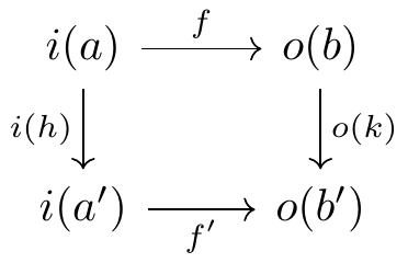
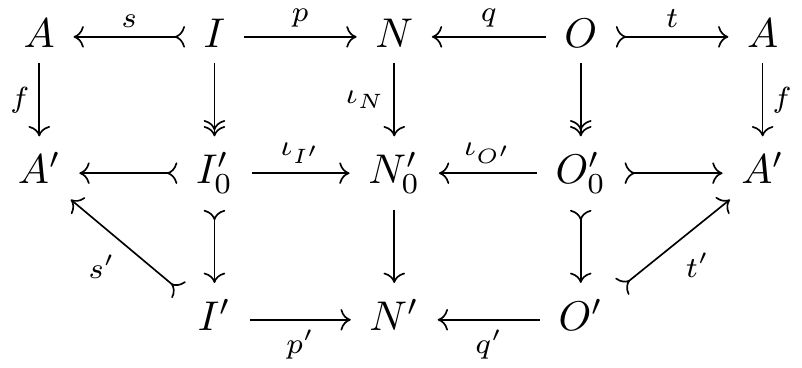
A generic cell in the double category of $F$-decorated cospans can be depicted as:

The laxators $\tilde\Gamma$ and unitors $\tilde\gamma$ of the lax double functor are used to define the external composition and identities in $\int F$. Given composable cospans $m = (a \rightarrow q \leftarrow b)$ and $n = (b \rightarrow r \leftarrow c)$, define $\Gamma_{m,n}$ to be the functor $$(F_1 \times_{F_0} F_1)(m,n) = \operatorname{apex}(\tilde F_1(m) \odot \tilde F_1(n)) \xrightarrow{\operatorname{apex}(\tilde\Gamma_{m,n})} \operatorname{apex}(\tilde F_1(m \odot n)) = F_1(m \odot n),$$ whose domain is the pullback in $\mathsf{Cat}$ of $F_1(m) \xrightarrow{\rho_m} F_0(b) \xleftarrow{\lambda_n} F_1(n)$. Then composition of decorated cospans is the operation: $$(a,x) \xrightarrow{(m,s)} (b,y) \xrightarrow{(n,t)} (c,z) \qquad\leadsto\qquad (m \odot n,\ \Gamma_{m,n}(s,t)).$$ Furthermore, the external composite of cells $(m,s) \xrightarrow{(\alpha,\nu)} (n,t)$ and $(o,u) \xrightarrow{(\beta,\pi)} (p,v)$ that satisfy $(\operatorname{ft}_R(\alpha), \rho_n(\nu)) = (\operatorname{ft}_L(\beta), \lambda_p(\pi))$ is $(\alpha \odot \beta,\ \Gamma_{n,p}(\nu,\pi))$. External identities are defined similarly using the functors $\gamma_a := \operatorname{apex}(\tilde\gamma_a)$ for $a \in \mathsf{A}$.

In case it got lost in the morass of notation, let us summarize the two key ways that this version of decorated cospans generalizes the existing one. First, and most importantly, the decorations allowed for a given cospan can depend on the whole cospan, not just on its apex. Second, the feet of the cospans (the objects of the double category) get their own decorations, which can be extracted from the cospan decorations by the transformations $\lambda$ and $\rho$. For two decorated cospans to be composable, not only must the feet of the cospans be compatible, so must be the decorations on the feet. In the langauge of the previous section, the first increase in generality is discarded by the lax double functor $\operatorname{Apex}: \mathbb{C}\mathsf{sp}(\mathsf{A}) \to \mathbb{M}(\mathsf{A},+)$ and the second is discarded by the double functor $\operatorname{coDisc}: \mathbb{M}(\mathsf{Cat},\times) \to \mathbb{S}\mathsf{pan}(\mathsf{Cat})$.

4 Examples

Any existing example of decorated cospans gives an example of the new formalism via the reductions above. So let’s see a few examples that actually need the extra generality afforded by the double Grothendieck construction.

4.1 The comma construction

In synthetic treatments of statistics and machine learning, a natural thing to consider is a small category, regarded as a theory in the sense of categorical logic, that is equipped with a distinguished morphism. Especially motivating to me are the statistical theories studied in my PhD thesis (Patterson 2020). A statistical theory consists of a small Markov category with some extra structure, specifying the constituents of a statistical model, plus a distinguished morphism $p: \theta \to x$, specifying its sampling distribution. My thesis viewed theories as objects and focused on morphisms of theories, which formally capture relationships between different theories. But statistical theories can also be viewed as themselves a kind of morphism, which can be composed to create hierarchical or multi-level statistical models. So, from the perspective of double categories, statistical theories should be understood not merely as objects in a category but as proarrows in a double category. A structurally similar story applies to neural networks in machine learning, where the distinguished morphism now plays the role of the prediction function.

Using comma categories and decorated cospans, we construct a double category whose proarrows consist of a cospan of categories together with a morphism in the apex category, such that its domain and codomain are images of objects in the left and right feet. Actually, to address my motivating examples in statistics or machine learning, we would need to use comma objects in a 2-category of categories with extra structure. For simplicity, we’ll just work with bare categories here.

Recall that the comma category of two functors $i: \mathsf{A} \to \mathsf{X}$ and $o: \mathsf{B} \to \mathsf{X}$ is the category $(i/o)$ having

• objects, a pair of objects $a \in \mathsf{A}$ and $b \in \mathsf{B}$ plus a morphism $f: i(a) \to o(b)$ in $\mathsf{X}$;
• morphisms $(a,b,f) \to (a',b',f')$, a pair of morphisms $h: a \to a'$ in $\mathsf{A}$ and $k: b \to b'$ in $\mathsf{B}$ inducing a commutative square in $\mathsf{X}$.

In addition, the comma category $(i/o)$ has evident projection functors $\pi_{\mathsf{A}}: (i/o) \to \mathsf{A}$ and $\pi_{\mathsf{B}}: (i/o) \to \mathsf{B}$.

The comma construction upgrades to a lax double functor, the comma double functor $$\operatorname{Comma}: \mathbb{C}\mathsf{sp}(\mathsf{Cat}) \to \mathbb{S}\mathsf{pan}(\mathsf{Cat}),$$ where $\operatorname{Comma}_0: \mathsf{Cat}\to \mathsf{Cat}$ is the identity functor and $\operatorname{Comma}_1: \mathsf{Cat}^\mathsf{Csp}\to \mathsf{Cat}^\mathsf{Span}$ sends a cospan $(\mathsf{A} \xrightarrow{i} \mathsf{X} \xleftarrow{o} \mathsf{B})$ to the span $(\mathsf{A} \xleftarrow{\pi_{\mathsf{A}}} (i/o) \xrightarrow{\pi_{\mathsf{B}}} \mathsf{B})$ and sends a map of cospans

to the map of spans

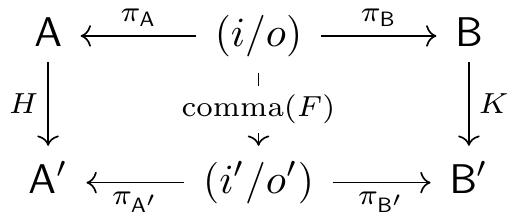
where the functor $\operatorname{comma}(F): (i/o) \to (i'/o')$ is defined by: $$\begin{aligned} (a, b, i(a) \xrightarrow{f} o(b)) &\mapsto (H(a), H(b), i'(H(a)) = F(i(a)) \xrightarrow{F(f)} F(o(b)) = o'(H(b))) \\ (h, k) &\mapsto (H(h), K(k)). \end{aligned}$$

For composable cospans $m = (\mathsf{A} \xrightarrow{i} \mathsf{X} \xleftarrow{o} \mathsf{B})$ and $n = (\mathsf{B} \xrightarrow{j} \mathsf{Y} \xleftarrow{p} \mathsf{C})$, the laxator is the feet-preserving map of spans whose apex map is the functor $$\begin{aligned} (i/o) \times_{\mathsf{B}} (j/p) &\to (\iota_{\mathsf{X}} \circ i / \iota_{\mathsf{Y}} \circ p) \\ (i(a) \xrightarrow{f} i(b), j(b) \xrightarrow{g} p(c)) &\mapsto (\iota_{\mathsf{X}} i(a) \xrightarrow{\iota_{\mathsf{X}} f} \iota_{\mathsf{X}} o(b) = \iota_{\mathsf{Y}} j(b) \xrightarrow{\iota_{\mathsf{Y}} g} \iota_{\mathsf{Y}} p(c)) \\ ((h,k), (k,\ell)) &\mapsto (h,\ell). \end{aligned}$$ Here $\iota_{\mathsf{X}}: \mathsf{X} \to \mathsf{X} +_{\mathsf{B}} \mathsf{Y}$ and $\iota_{\mathsf{Y}}: \mathsf{Y} \to \mathsf{X} +_{\mathsf{B}} \mathsf{Y}$ are the coprojections associated with the pushout of categories. Finally, for each category $\mathsf{A}$, the unitor is the feet-preserving map of spans whose apex map is the functor $\mathsf{A} \to (\operatorname{id}_{\mathsf{A}} / \operatorname{id}_{\mathsf{A}}) \cong {\mathsf{A}}^{\rightarrow}$ that sends $a \in \mathsf{A}$ to $(a,a,\operatorname{id}_a)$ and $h: a \to a'$ to $(h,h)$.

The Grothendieck construction $\int \operatorname{Comma}$ is a double category that has:

• objects, a small category $\mathsf{A}$ together with an object $a \in \mathsf{A}$;
• arrows $(\mathsf{A}, a) \to (\mathsf{A}', a')$, a functor $H: \mathsf{A} \to \mathsf{A}'$ together with a morphism $h': H(a) \to a'$ in $\mathsf{A}'$;
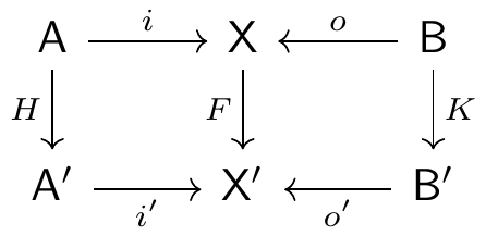
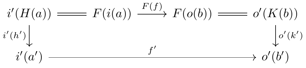
• proarrows with source $(\mathsf{A}, a)$ and target $(\mathsf{B}, b)$, a cospan of categories $m = (\mathsf{A} \xrightarrow{i} \mathsf{X} \xleftarrow{o} \mathsf{B})$ together with a morphism $f: i(a) \to o(b)$ in $\mathsf{X}$;
• cells $(m,f) \to (m',f')$ with source $(H,h')$ and target $(K,k')$, a map of cospans $(H,F,K)$ as depicted above such that the following square commutes:

External composition is given by pushout of categories, followed by composition in the quotient category.

When transplanted to the setting of Markov categories, such a cell is a refinement of what I have called a lax morphism of statistical theories (Patterson 2020, sec. 3.5).

4.2 Graphs with dangling edges

Directed graphs with dangling edges are an intuitively simple concept that is surprisingly resistant to clean mathematical treatment. One elegant approach, suited to the combinatorics of properads, has been developed by Joachim Kock (Kock 2016). In this approach, a dangling-edge graph (called by Kock simply a “graph”) is a diagram of finite sets

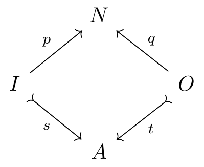
where the functions $s$ and $t$ are injective. The elements of $N$ are the nodes or vertices of the graph and the elements of $A$ are the arcs or edges. An edge in the image of $s$ has a source node, which is given by $p$; otherwise, the edge is incoming. Similarly, an edge in the image of $t$ has a target node, which is given by $q$; otherwise, the edge is outgoing. An edge that is incoming or outgoing (or both) is called dangling, and an edge that is incoming and outgoing is called passing. A dangling-edge graph that has no nodes, and which therefore has only passing edges, is called a shrub.

Dangling-edge graphs are evidently a subset of the objects of a copresheaf category. A morphism of dangling-edge graphs is a morphism in this copresheaf category, i.e., a commutative diagram:

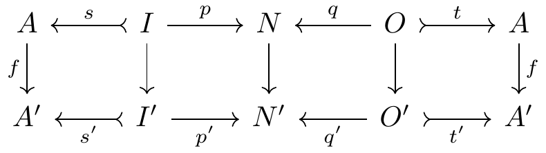
The category of dangling-edge graphs is denoted $\mathsf{DGraph}$.

We are going to construct a double category whose objects are finite sets, regarded as shrubs, and whose proarrows are dangling-edge graphs with specified incoming and outgoing edges. Composition of proarrows will glue outgoing edges of the first graph to incoming edges of the second graph. To do this construction, we’ll need the edge-analogue of the functor that sends a finite set $V$ to the category of graphs with vertex set $V$. Unfortunately, the injectivity condition in dangling-edge graphs causes complications.

Let $\operatorname{Arc}: \mathsf{FinSet}\to \mathsf{Cat}$ be the functor that sends a finite set $A$ to the category of dangling-edge graphs with edge set $A$. The morphisms in this category are edge-preserving morphisms of dangling-edge graphs, whose $I$ and $O$ components are necessarily injective. For any function $f: A \to A'$, the functor $\operatorname{Arc}(f)$ is defined in terms of the following commutative diagram.

This requires some explanation. Given a dangling-edge graph $G \in \operatorname{Arc}(A)$, we construct another dangling-edge graph $\operatorname{Arc}(f)(G) \in \operatorname{Arc}(A')$ by taking the epi-mono factorizations of $f \circ s$ and $f \circ t$, which define $I_0'$ and $O_0'$ respectively, and then taking $N_0'$ to be the colimit of the diagram of finite sets: $$I_0' \twoheadleftarrow I \xrightarrow{p} N \xleftarrow{q} O \twoheadrightarrow O_0'.$$ In effect, we take the edges $a' \in A'$ to be incoming or outgoing whenever possible—whenever $a'$ is not in the image of $f \circ s$ or $f \circ t$—and then we quotient the nodes as freely as possible to obtain a morphism $G \to \operatorname{Arc}(f)(G)$ in $\mathsf{DGraph}$. The functor $\operatorname{Arc}(f)$ also acts on morphisms in $\operatorname{Arc}(A)$, the description of which we omit. The functorality of $\operatorname{Arc}: \mathsf{FinSet}\to \mathsf{Cat}$ follows from the uniqueness of epi-mono factorizations and colimits. Actually, since this uniqueness holds only up to unique isomorphism, $\operatorname{Arc}$ is a pseudofunctor, but we aren’t going to worry about that.

The functor $\operatorname{Arc}: \mathsf{FinSet}\to \mathsf{Cat}$ has the desirable property that any morphism $\phi: G \to G'$ of dangling-edge graphs with component $f := \phi_A: A \to A'$ factorizes as $$G \to \operatorname{Arc}(f)(G) \to G',$$ where the latter morphism belongs to $\operatorname{Arc}(A')$:

To see this, note that if $I \twoheadrightarrow I_0' \rightarrowtail I'$ is the epi-mono factorization of $\phi_I: I \to I'$, then post-composing with $s'$ gives the epi-mono factorization of $s' \circ \phi_I = f \circ s$, and similarly for the $O$ component. The function is $N_0' \to N'$ is then given by the universal property of the colimit $N_0'$.

Another complication is that to compose dangling-edge graphs, we must restrict to cospans with monic legs. Given a finitely cocomplete category $\mathsf{A}$ with monomorphisms stable under pushout, such as a topos, let $\mathbb{C}\mathsf{sp}_{\mathrm{m}}(\mathsf{A})$ be the double of category of cospans in $\mathsf{A}$ whose legs are monic. Its cells are the usual maps of cospans, with no assumption of monicness. Thus, the double category has $\mathbb{C}\mathsf{sp}_{\mathrm{m}}(\mathsf{A})_0 = \mathsf{A}$ and $\mathbb{C}\mathsf{sp}_{\mathrm{m}}(\mathsf{A})_1 = \mathsf{A}^{\mathsf{Csp}_{\mathrm{m}}}$, where ${\mathsf{Csp}_{\mathrm{m}}}:= \{\bullet \rightarrowtail \bullet \leftarrowtail \bullet\}$ is the walking cospan with monic legs (formally, a finite limits theory).

With these preliminaries aside, we define a lax double functor $$F: \mathbb{C}\mathsf{sp}_{\mathrm{m}}(\mathsf{FinSet}) \to \mathbb{M}(\mathsf{Cat},\times)$$ with $F_0: \mathsf{FinSet}\xrightarrow{!} \mathsf{1}$ the unique map and $F_1: \mathsf{FinSet}^{\mathsf{Csp}_{\mathrm{m}}}\to \mathsf{Cat}$ the following functor. On objects, $F_1$ sends a cospan $m = (A_i \xrightarrow{i} A \xleftarrow{o} A_o)$ to the category of dangling-edge graphs with edge set $A$, such that the legs $i$ and $o$ inject into the sets of incoming and outgoing edges, respectively. Importantly, this condition refers to the whole cospan, not just its apex! The category $F_1(m)$ is a full subcategory of $\operatorname{Arc}(A)$. On morphisms, $F_1$ sends a map of cospans $\alpha = (f_i, f, f_o): m \to m'$ to the functor $F_1(\alpha): F_1(m) \to F_1(m')$ given by (co)restriction of $\operatorname{Arc}(f): \operatorname{Arc}(A) \to \operatorname{Arc}(A')$.

Finally, we define the laxators and unitors of the lax double functor $F$. Write $L: \mathsf{FinSet}\to \mathsf{DGraph}$ for the functor that sends a finite set $A$ to the shrub with edge set $A$. For composable cospans $m = (A_i \rightarrow A \leftarrow S)$ and $n = (S \rightarrow B \leftarrow B_o)$ in $\mathsf{FinSet}^{\mathsf{Csp}_{\mathrm{m}}}$, the laxator $$\Gamma_{m,n}: F_1(m) \times F_1(n) \to F_1(m \odot n), \quad (G,H) \mapsto G +_{L(S)} H$$ takes the pushout in $\mathsf{DGraph}$ along the shrub $L(S)$. Conveniently, Kock has already shown that such pushouts in $\mathsf{DGraph}$ exist and are computed pointwise (Kock 2016, Proposition 1.5.2). Thus, the dangling-edge graph $\Gamma_{m,n}(G,H)$ has edge set $A +_S B$ and other sets given by coproduct. Similarly, the action of $\Gamma_{m,n}$ on cells is by coproduct. For each finite set $S$, the unitor $$\gamma_S: 1 \to F_1(S), \quad * \mapsto L(S)$$ picks out the corresponding shrub.

The double category of dangling-edge graphs is the Grothendieck construction of the lax double functor $\mathbb{C}\mathsf{sp}_{\mathrm{m}}(\mathsf{FinSet}) \xrightarrow{F} \mathbb{M}(\mathsf{Cat},\times) \xrightarrow{\operatorname{coDisc}} \mathbb{S}\mathsf{pan}(\mathsf{Cat})$. The proarrows are dangling-edge graphs with chosen incoming and outgoing edges, and the cells are arbitrary morphisms of dangling-edge graphs together with compatible maps of the incoming and outgoing edges.

If the injectivity constraint in dangling-edge graphs is dropped, one obtains a structure isomorphic to whole-grain Petri nets (Kock 2022). A double category of whole-grain Petri nets with chosen incoming and outgoing transitions can be constructed similarly to that of dangling-edge graphs. In fact, the construction is much simpler because we can work in a copresheaf category.

5 Discussion

As noted in the previous post, there is a logical gap between our double Grothendieck construction, which assumes the double category is strict, and its application to decorated cospans, using the pseudo double category of cospans. This discrepancy could be resolved by strictifying or, better, by appropriate use of 2-categorical ideas.

Both of our examples should be not only double categories but monoidal double categories, with monoidal product derived from the coproduct. The principled way to address this would be to derive the Grothendieck construction for monoidal double categories, as hinted at last time, and apply it to $(\mathbb{C}\mathsf{sp}(\mathsf{A}), +)$, the monoidal double category of cospans. I would expect that a lax monoidal functor $F: (\mathsf{A},+) \to (\mathsf{Cat},\times)$ gives rise to a lax monoidal double functor $\tilde F: (\mathbb{C}\mathsf{sp}(\mathsf{A}),+) \to (\mathbb{S}\mathsf{pan}(\mathsf{Cat}),\times)$, which would extend the connection to decorated cospans explained here.

References

Baez, John C., Kenny Courser, and Christina Vasilakopoulou. 2022. “Structured Versus Decorated Cospans.” Compositionality 4 (3). https://doi.org/10.32408/compositionality-4-3.

Fong, Brendan. 2015. “Decorated Cospans.” Theory and Applications of Categories 30 (33): 1096–1120. http://www.tac.mta.ca/tac/volumes/30/33/30-33abs.html.

Kock, Joachim. 2016. “Graphs, Hypergraphs, and Properads.” Collectanea Mathematica 67 (2): 155–90. https://doi.org/10.1007/s13348-015-0160-0.

———. 2022. “Whole-Grain Petri Nets and Processes.” Journal of the ACM 70 (1): 1–58. https://doi.org/10.1145/3559103.

Patterson, Evan. 2020. “The Algebra and Machine Representation of Statistical Models.” PhD thesis, Stanford University. https://arxiv.org/abs/2006.08945.

———. 2023. “Structured and Decorated Cospans from the Viewpoint of Double Category Theory.” In Applied Category Theory 2023. https://arxiv.org/abs/2304.00447.