Neural wiring diagrams for message passing in multiscale organizations

Abstract

In our recent paper, “Dynamic task delegation for hierarchical agents”, Sophie Libkind and I described a task delegation from an agent to a team of subordinates as morphisms in a certain operad called $\mathbb{O}\mathbf{rg}_{\mathfrak{m}}$. However, such morphisms include a great deal of data, and the examples we gave there barely scratched the surface of what’s possible. In this post I’ll show how “recumbent” neural wiring diagrams—with arbitrary feedback and “axon” splitting—give rise to a message-passing language for describing certain such task delegations. That is, I’ll define a cyclic operad $\mathbf{rnWD}$ and a functor $\mathbf{rnWD}\to\mathbb{O}\mathbf{rg}_{\mathfrak{m}}$.

Edit

The arXiv paper that this post cites contains an error, and had to be taken down for the time being. However, the math in this post still stands.¹

1 Introduction

In our recent paper, “Dynamic task delegation for hierarchical agents”,² Sophie Libkind and I described what we called task delegations, procedures involving an agent and a team of subordinates, as the morphisms in a certain operad $\mathbb{O}\mathbf{rg}_\mathfrak{m}$. Think of agents as things that perform tasks, like travel agents, agent 007, and cleaning agents: you give the agent a task of some type, and it comes back to you with an outcome.

We formalize this in terms of what we call “task-solution interfaces”, but which I want to call portfolios. A portfolio consists of a set $T$ of tasks and for each task $t:T$ a set $O(t)$ of possible outcomes for that task. Then an agent $A$ is understood as something connecting one portfolio—the set of tasks that $A$ can be assigned—to a bunch of portfolios, one for each of $A$’s subordinates. The agent $A$ itself is intuitively an “evolving planner”: it performs a task $t$ by planning how to orchestrate its subordinates in solving their own subtasks and using those solutions to choose new subtasks for them to solve, repeatedly, until principal agent $A$ is ready to determine an outcome $o:O(t)$. Once this task is solved, $A$ can “evolve” in the sense that it can update how it will plan tasks in the future.

Sophie and I formalized all of this is formalized using the theory of polynomial functors. A portfolio is a polynomial $p=\sum_{t:T}\mathcal{y}^{O(t)}$; these are the objects, and agents are the morphisms, in a category-enriched operad $\mathbb{O}\mathbf{rg}_\mathfrak{m}$. The morphisms are given by the formula $$\mathbb{O}\mathbf{rg}_\mathfrak{m}(q_1,\ldots,q_k; p)\coloneqq[p,\mathfrak{m}_{q_1 +\cdots+ q_k}]\textnormal{-}\mathbf{Coalg}$$ where $\mathfrak{m}\colon\mathbf{Poly}\to\mathbf{Poly}$ is the free monad monad, $[-,-]$ is an inner hom, and $h\textnormal{-}\mathbf{Coalg}$ is the category of coalgebras for a polynomial $h$. If you’re reeling from either the weight of all that notation or from the sheer amount of data in such a thing, this is normal. On the one hand, it makes sense: there should be a lot of room within the realm of all “evolving planners,” so $\mathbb{O}\mathbf{rg}_\mathfrak{m}$ has to package all that. On the other hand, we need intuition for what sorts of things we can say in this language.

In this blog post, I’ll show how recumbent wiring diagrams give a way to visualize cases of such hierarchical planning, though they are still relatively simple compared to what’s possible. Recumbent string diagrams were those used by Joyal and Street in their seminal work on string diagrams, though I learned about them from Delpeuch and Vicary. Let’s begin there, then move on to how they connect to my work with Sophie, then generalize to add wire-splitting and feedback, and finally conclude.

2 The operad of recumbent wiring diagrams

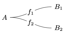
Recumbent string diagrams in the sense of Joyal and Street are graphs embedded in the plane, which look as shown on the left; I’d usually draw them as wiring diagrams, as shown to the right:

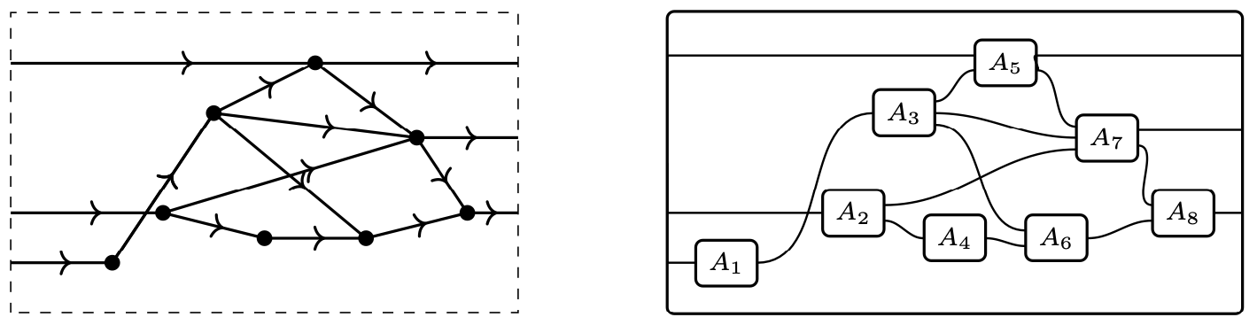
The thing to notice about the graph is that none of the wires go backwards, and that no two vertices project to the same point on the $x$-axis; this is the “recumbency” requirement. In terms of computations, this says that no two computations take place at the same time.

There are a couple of differences between string diagrams and wiring diagrams. First, string diagrams were presented as topological and embedded in the plane, whereas wiring diagrams were presented as combinatorial and just about connectivity. Second, string diagrams do not include an outer box, because they are understood as being built up from monoidal product and composition, whereas wiring diagrams do include the outer box, because they are understood as morphisms $\varphi\colon A_1\ldots,A_k\to B$ in an colored operad and the outer box is the codomain $B$. In this post, we’ll take an operadic viewpoint, but we’ll need the recumbency condition from Joyal and Street: not the topology, but the fact that no two vertices / boxes occur at the same time.

The operad of wiring diagrams for symmetric monoidal categories is the story of how you can nest whole wiring diagrams into boxes. Indeed, the objects in this (colored) operad are the box shapes, the morphisms are the wiring diagrams, and placing a wiring diagram into a box is composition. Recumbent wiring diagrams also form an operad, one that’s much easier to write down, as I’ll now explain.

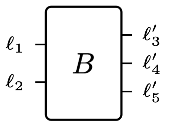
Fix a set $L$ of “wire labels”; a finite $L$-set is a pair $(A,\ell)$, where $A$ is a finite set $A$ and $\ell\colon A\to L$ picks a label for each $a:A$. We define a box to be a pair $B=(B^{\textnormal{in}},B^{\textnormal{out}})$ of finite $L$-sets. For example, $B^{\textnormal{in}}=(\{1,2\},\ell)$ and $B^{\textnormal{out}}=(\{3,4,5\},\ell')$ would be drawn

A recumbent wiring diagram (or WD), denoted $\varphi\colon A_1,\ldots,A_n\to B$, is defined as a list $W_1,\ldots,W_n$ of finite $L$-sets together with $L$-preserving bijections $$\begin{aligned} \tag{rWD} \varphi_i\colon W_i+A_i^{\textnormal{out}}&\xrightarrow[]{\cong} A_{i+1}^{\textnormal{in}}+W_{i+1} \end{aligned}$$ for each $0\leq i\leq n$, where $W_0\coloneqq \varnothing$ and $W_{n+1}\coloneqq \varnothing$ and $A_0^{\textnormal{out}}\coloneqq B^{\textnormal{in}}$ and $A_{n+1}^{\textnormal{in}}=B^{\textnormal{out}}$. That all sounds confusing but let me rewrite it in case $n=3$: $$\begin{aligned} \varphi_0\colon B^{\textnormal{in}}&\xrightarrow[]{\cong} A_1^{\textnormal{in}}+W_1\\ \varphi_1\colon W_1+A_1^{\textnormal{out}}&\xrightarrow[]{\cong} A_2^{\textnormal{in}}+W_2\\ \varphi_2\colon W_2+A_2^{\textnormal{out}}&\xrightarrow[]{\cong} A_3^{\textnormal{in}}+ W_3\\ \varphi_3\colon W_3+A_3^{\textnormal{out}}&\xrightarrow[]{\cong} B^{\textnormal{out}} \end{aligned}$$ The idea is that the $W_i$ represent the extra wires that are present at the same time as box $a_i$.

Let’s do an example, but with one label $L=1$ to avoid having to consider labels.

There is one additional wire present during $A_1$ and another additional wire present during $A_2$, so we have $W_1=1$, $W_2=1$, and $W_3=0$. Here $A_0^{\textnormal{out}}=B^{\textnormal{in}}=2$, $A_0^{\textnormal{in}}=B^{\textnormal{out}}=1$, $A_1^{\textnormal{in}}=1$, $A_1^{\textnormal{out}}=2$, $A_2^{\textnormal{in}}=2$, $A_2^{\textnormal{out}}=1$, $A_3^{\textnormal{in}}=2$, and $A_3^{\textnormal{out}}=1$. And we have the desired bijections $$2\cong 1+1,\qquad 1+2\cong2+1,\qquad 1+1\cong2+0,\qquad 0+1\cong1.$$

Recumbent wiring diagrams (with labels in $L$) can be substituted in an obvious way, so they form a multicategory, also known as a nonsymmetric colored operad. We’ll denote it $\mathbf{rWD}_L$.

3 Recumbent WDs as message passing plans

In my work with Sophie, we were interested in evolving planners, but in this section we’ll take the “evolution” out of it. We’ll see that for any function $X\colon L\to\mathbf{Set}$, there is a map of multicategories $$\tag{MP} \mathit{MP}_X\colon\mathbf{rWD}_L\to\mathbb{O}\mathbf{rg}_\mathfrak{m}$$ The idea is that a recumbent wiring diagram gives a message passing plan, which is a morphism in $\mathbb{O}\mathbf{rg}_\mathfrak{m}$. In fact, it’s an especially simple sort of morphism. Namely, the morphisms that arise via the “message passing” functor $\mathit{MP}_X$ will be constant: the corresponding coalgebra only has one state, so as mentioned there is no evolution involved. Second, these morphisms will not use the monoidal product $\vee$ but instead the much simpler monoidal product $+$. Recall that $p\vee q=p+(p\otimes q)+q$, which allows one or more things to happen simultaneously. Clearly there is a map $p+q\to p\vee q$, which avoids all simultaneity. In other words, these planners only talk to one of their subordinates at a time. In case it wasn’t clear, this corresponds to the recumbency requirement.

So how does $\mathit{MP}_X$ work? Before we answer that, let’s simplify the target category a bit. Let $\mathbf{Poly}_\mathfrak{m}$ denote the Kleisli category of the free monad monad $\mathfrak{m}\colon\mathbf{Poly}\to\mathbf{Poly}$. Its objects are polynomials and a map $p\to q$ is a natural transformation $p\to\mathfrak{m}_q$. To each position (task) $P:p(1)$, it assigns a flowchart of $q$-tasks, and then returns the result as an outcome in $p[P]$. This is the category that Harrison Grodin called the category of poly-morphic effect handlers. Coproducts in $\mathbf{Poly}$ lift to coproducts in $\mathbf{Poly}_\mathfrak{m}$, so we can consider the operad whose morphisms are of the form $$\varphi\colon p\to\mathfrak{m}_{q_1+\cdots+q_k},$$ and we again denote this $\mathbf{Poly}_\mathfrak{m}$. The idea is that $\varphi$ assigns each task in $p$ a flowchart of tasks from different $q_i$’s, one at a time.

There is an identity-on-objects inclusion $\mathbf{Poly}_\mathfrak{m}\to\mathbb{O}\mathbf{rg}_\mathfrak{m}$ that includes such $\varphi$ as the constant coalgebras $1\to[p,\mathfrak{m}_{q_1+\cdots+q_k}](1)$, so to obtain a map of operads as in (MP), it suffices to find an operad functor $$\mathit{MP}_X\colon\mathbf{rWD}_L\to\mathbf{Poly}_\mathfrak{m}.$$ So again, we ask how does this functor work? First we’ll give the full technicalities and then give a simple example; the reader can feel free to skip to right around the diagram (myWD) below. So here go the technical details. Let’s begin with how $\mathit{MP}_X$ works objects.

Recall that a box is a pair $((A,\ell),(A',\ell'))$ of finite $L$-sets. For each $a\in A$, let $X_a\coloneqq X(\ell(a))$ and, for $a'\in A'$, let $X_{a'}\coloneqq X(\ell'(a')$. Then the functor $\mathit{MP}_X$ sends that box to the polynomial $$\mathit{MP}_X((A,\ell),(A',\ell'))\coloneqq\Big(\prod_{a\in A}X_a\Big)\mathcal{y}^{\,\prod_{a'\in A'}X_{a'}}$$ For example, if the box has two wires on the left and one on the right, with associated sets $\mathbb{N},\mathbb{Z}$ and $\mathbb{R}$, then $\mathit{MP}_X$ will send it to $(\mathbb{N}\times\mathbb{Z})\mathcal{y}^\mathbb{R}$.

Let’s move on to morphisms. Suppose that $a_1,\ldots,a_n,b$ are boxes and that $\varphi\colon a_,\ldots,a_n\to b$ is a recumbent wiring diagram given by finite $L$-sets $W_1,\ldots,W_n$ and bijections $\varphi_0,\ldots\varphi_n$, as in [rWD]. These give rise to bijections $$\begin{aligned} \prod_{b:B}X_b&\cong\prod_{a: A_1}X_a\times\prod_{w: W_1}X_w\\ \prod_{w: W_i}X_w\times\prod_{a':A_i'}X_{a'}&\cong\prod_{a: A_{i+1}}X_a\times\prod_{w: W_{i+1}}X_w&(1\leq i<n)\\ \prod_{w: W_n}X_w\times\prod_{a':A_n'}X_{a'}&\cong\prod_{b': B'}X_{b'} \end{aligned}$$ These in turn give rise to projection maps $$\begin{aligned} \prod_{b:B}X_b&\to\prod_{a: A_1}X_a\\ \prod_{b:B}X_b\times\prod_{j=1}^i\prod_{a':A_j'}X_{a'}&\to\prod_{a:A_{j+1}}X_a&(1\leq i<n)\\ \prod_{b:B}X_b\times\prod_{j=1}^n\prod_{a':A_j'}X_{a'}&\to\prod_{b':B'}X_{b'} \end{aligned}$$ These immediately give rise to a map of polynomials $$\begin{aligned} \Big(\prod_{b: B}X_b\Big)\mathcal{y}^{\,\prod_{b': B'}X_{b'}}&\longrightarrow \Big(\prod_{a: A_1}X_a\Big)\mathcal{y}^{\,\prod_{a': A'_1}X_{a'}} \triangleleft\cdots\triangleleft \Big(\prod_{a: A_n}X_a\Big)\mathcal{y}^{\,\prod_{a': A'_n}X_{a'}}\\&\longrightarrow \mathfrak{m}_{\sum_{i=1}^n\Big(\prod_{a: A_i}X_a\Big)\mathcal{y}^{\,\prod_{a': A'_i}X_{a'}}} \end{aligned}$$ and hence the required map of polynomials $$\mathit{MP}_X(\varphi)\colon\mathit{MP}_X(b)\to\mathfrak{m}_{\mathit{MP}_X(a_1)+\cdots+\mathit{MP}_X(a_n)}.$$

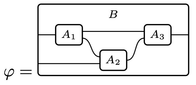
While the above few paragraphs may be a bit technical for a blog post, one sees that to turn a recumbent wiring diagram into the required map of polynomials is really just a matter of putting isomorphisms and projections together. But perhaps we can clarify a bit more what’s happening on a simple recumbent wiring diagram $\varphi\colon T_1,T_2\to U$ such as the following:

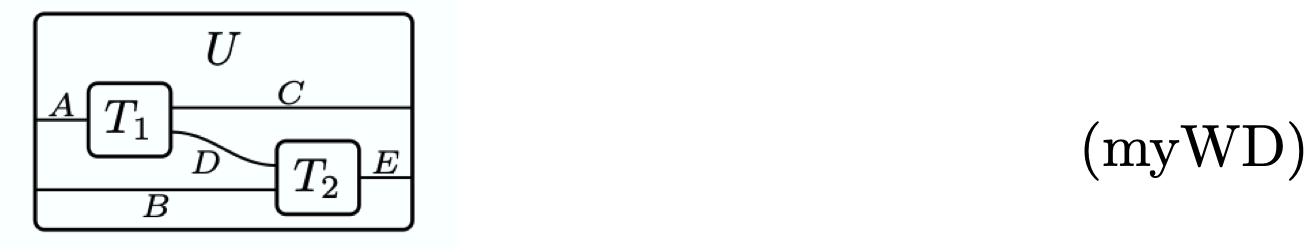
We’ll use the labels $A,\ldots,E$ to also denote the sets assigned by $X$, and we’ll use juxtaposition to denote products, e.g. $AB$ means $A\times B$. Then $\mathit{MP}_X(\varphi)$ is supposed to be a map of polynomials $$(AB)\mathcal{y}^{CE}\to \mathfrak{m}_{A\mathcal{y}^{CD}+DB\mathcal{y}^E}$$ Since there’s always a map $p\triangleleft q\to \mathfrak{m}_{p+q}$, it suffices to find a map of polynomials $$(AB)\mathcal{y}^{CE}\to A\mathcal{y}^{CD}\triangleleft DB\mathcal{y}^E$$ and this is the same as three maps $$AB\to A,\qquad ABCD\to DB,\;\text{and}\qquad ABCDE\to CE$$ all of which we can take to be projections. Now what do all these projections mean in terms of the diagram in (myWD)?

On the left side of the surrounding box, we have two wires $A$ and $B$, so an element of the product set $AB$ “comes in” on the left. Its first projection to $A$ is delivered to the box $a_1$. Then, an output of that box is of the form $CD$, so now we have $ABCD$ at our disposal, and projection gives rise to inputs of the form $DB$ which are delivered to the second box. Then, an output of that box is of the form $E$, so we now have $ABCDE$ at our disposal, and projection gives rise to an element of the form $CE$ which is delivered to the right side of the surrounding box.

But we can do better with less work.

4 A cyclic operad of recumbent “neural” WDs

In this section we’ll see that we can get what we might call neural wiring diagrams,

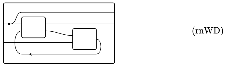
diagrams with splitting and feedback, by simply relieving ourselves of constraints we never used! For example, nothing in the definition of $\mathit{MP}_X$ needed the maps in (rWD) to be bijections; what we actually used were functions $$\varphi_i\colon A_{i+1}^{\textnormal{in}}+W_{i+1}\to W_i+A_i^{\textnormal{out}}$$ in the direction of the inverses of the isomorphisms shown. We also can dispense with labels $L$ and the function $X\colon L\to\mathbf{Set}$ and use polynomials to represent collections of wires. The polynomial $p=\mathcal{y}^A+\mathcal{y}^B$ can be used to represent two wires, one carrying set $A$ and one carrying set $B$. We want to imagine those two wires together carrying elements of type $A\times B$, and this is exactly the set $\Gamma(p)=\mathbf{Poly}(p,\mathcal{y})=A\times B$ of $p$’s “global sections”. Note that the global sections functor is contravariant and strong monoidal: $$\Gamma\colon(\mathbf{Poly}^\textnormal{op},0,+)\longrightarrow(\mathbf{Set},1,\times)$$

So a polynomial $p=\sum_{w:W}\mathcal{y}^{p[w]}$ represents a set $W$ of wires, and for each wire $w:W$, a set $p[w]$ that the wire is “carrying”. A map of polynomials $\varphi\colon q\to p$ sends each $q$-wire $x$ to a $p$-wire $w\coloneqq\varphi_1(w)$ as well as a function $\varphi^\sharp_v\colon p[w]\to q[v]$. For example, if $p=\mathcal{y}^A$ and $q=\mathcal{y}^{B_1}+\mathcal{y}^{B_2}$, then such a map $\varphi$ would be given by two functions $f_1\coloneqq \varphi_1^\sharp\colon A\to B_1$ and $f_2\coloneqq \varphi_2^\sharp\colon A\to B_2$, which we could draw this way

With this technology, we can describe recumbent neural wiring diagrams as forming a cyclic operad $\mathbf{rnWD}$. An object is a pair $(p^{\textnormal{in}},p^{\textnormal{out}})$ of polynomials, representing a box with input ports $p^{\textnormal{in}}$ and output ports $p^{\textnormal{out}}$. For any $K:\mathbb{N}$, a $K$-ary morphism $$(p_1^{\textnormal{in}},p_1^{\textnormal{out}}),\ldots,(p_K^{\textnormal{in}},p_K^{\textnormal{out}})\to(q^{\textnormal{in}},q^{\textnormal{out}})$$ is going to represent a recumbent neural wiring diagram. For example we will be able to represent this diagram

as a map $\Phi\colon(p_1^{\textnormal{in}},p_1^{\textnormal{out}}),(p_2^{\textnormal{in}},p_2^{\textnormal{out}})\to (q^{\textnormal{in}},q^{\textnormal{out}})$, where $$\begin{aligned} p_1^{\textnormal{in}}&\coloneqq \mathcal{y}^A+\mathcal{y}^E& p_1^{\textnormal{out}}&\coloneqq\mathcal{y}^C+\mathcal{y}^D\\ p_2^{\textnormal{in}}&\coloneqq \mathcal{y}^D+\mathcal{y}^{B'}& p_2^{\textnormal{out}}&\coloneqq\mathcal{y}^E\\ q^{\textnormal{in}}&\coloneqq \mathcal{y}^A+\mathcal{y}^B& q^{\textnormal{out}}&\coloneqq\mathcal{y}^A+\mathcal{y}^C+\mathcal{y}^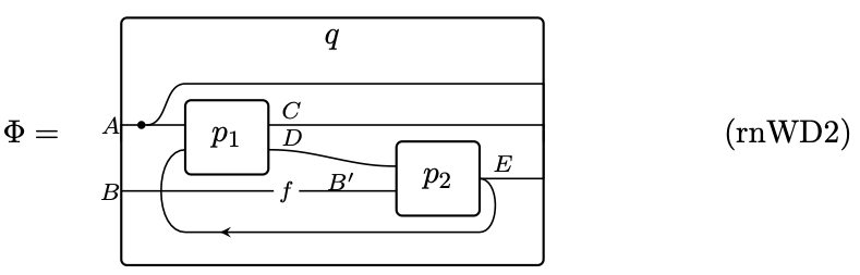E \end{aligned}$$ To see how, we need to define the maps in the cyclic operad $\mathbf{rnWD}$. They are actually pretty simple: we pick a few (in this case three) polynomials to represent the extra wires that hold values while various boxes are firing, and then we write down a bunch of polynomial morphisms to say how the wires relate from one time step to the next.

So the idea is that we can use these to define agents in the sense of my paper with Sophie. Whereas for an arbitrary agent in $\mathbb{O}\mathbf{rg}_\mathfrak{m}$, the agent has a great deal of control over the way information is passed between its subordinates, an agent arising via the functor $\mathit{MP}$ always has its subagents pass messages according to the wiring diagram (rnWD2). The only thing these simpler agents do is to hold state, namely whatever is currently in the feedback wires. Let’s get into it.

Recall that for any $K\geq 0$, the cyclic group $\mathbb{Z}/(K+1)$ has elements $\{0,\ldots,K\}$ which add according to modular arithmetic, e.g. $0+1=1$ and $K+1=0$. Now we can define the maps as follows: $$\begin{aligned} \mathbf{rnWD}&((p_1^{\textnormal{in}},p_1^{\textnormal{out}}),\ldots,(p_K^{\textnormal{in}},p_K^{\textnormal{out}});(q^{\textnormal{in}},q^{\textnormal{out}}))\coloneqq\quad \text{let $p_0^{\textnormal{in}}\coloneqq q^{\textnormal{out}}$ and $p_0^{\textnormal{out}}\coloneqq q^{\textnormal{in}}$ in}\\\\& \sum_{w\colon\{0,\ldots,K\}\to\mathop{\mathrm{Ob}}(\mathbf{Poly})}\;\sum_{k:\mathbb{Z}/(K+1)} \mathbf{Poly}\left(p_{k+1}^{\textnormal{in}}+w_{k+1},\,w_k+p_k^{\textnormal{out}}\right) \end{aligned}$$ For the diagram (rnWD2), there are $K=2$ inner boxes, $w_0\coloneqq\mathcal{y}^E$ represents the feedback wire, $w_1\coloneqq\mathcal{y}^A+\mathcal{y}^B$ represents the (forward-going) wires holding values while $p_1$ is firing, and $w_2\coloneqq\mathcal{y}^A+\mathcal{y}^C$ represents the (forward-going) wires holding values while $p_2$ is firing. We invite the reader to use (rnWD2), which includes some function $f\colon B\to B'$, to guess the maps $$\begin{aligned} (\mathcal{y}^A+\mathcal{y}^E)+(\mathcal{y}^A+\mathcal{y}^B)&\longrightarrow(\mathcal{y}^E)+(\mathcal{y}^A+\mathcal{y}^B)\\ (\mathcal{y}^D+\mathcal{y}^{B'})+(\mathcal{y}^A+\mathcal{y}^C)&\longrightarrow(\mathcal{y}^A+\mathcal{y}^B)+(\mathcal{y}^C+\mathcal{y}^D)\\ (\mathcal{y}^A+\mathcal{y}^C+\mathcal{y}^E)+(\mathcal{y}^E)&\longrightarrow(\mathcal{y}^A+\mathcal{y}^C)+(\mathcal{y}^E) \end{aligned}$$ corresponding to $k=0,1,2$. Anyone who knows polynomial maps will not find these difficult to guess without even checking the diagram, but then can use the diagram to verify that it all makes sense.

So we’ve now seen that polynomials give a very compact way to represent recumbent neural wiring diagrams. But the point is that these can be used to represent some morphisms in $\mathbb{O}\mathbf{rg}_\mathfrak{m}$. That is, we will now construct a functor $$\mathit{MP}\colon\mathbf{rnWD}\to\mathbb{O}\mathbf{rg}_\mathfrak{m}.$$ This functor on objects is given by $(p^{\textnormal{in}},p^{\textnormal{out}})\mapsto \Gamma(p^{\textnormal{in}})\mathcal{y}^{\Gamma(p^{\textnormal{out}})}$. We’ll denote this latter polynomial as follows: $$\begin{pmatrix}p^{\textnormal{out}}\\p^{\textnormal{in}}\end{pmatrix}\coloneqq\begin{bmatrix}\Gamma(p^{\textnormal{out}})\\\Gamma(p^{\textnormal{in}})\end{bmatrix}=\Gamma(p^{\textnormal{in}})\mathcal{y}^{\Gamma(p^{\textnormal{out}})}$$ Where does $\mathit{MP}$ send a morphism $\Phi\colon(p_1^{\textnormal{in}},p_1^{\textnormal{out}}),(p_2^{\textnormal{in}},p_2^{\textnormal{out}})\to (q^{\textnormal{in}},q^{\textnormal{out}})$? Again, let $p_0^{\textnormal{in}}\coloneqq q^{\textnormal{out}}$ and $p_0^{\textnormal{out}}\coloneqq q^{\textnormal{in}}$, and suppose $\Phi=(w,\varphi)$, where for each $k\in\{0,\ldots,K\}$, we write $w_k\in\mathop{\mathrm{Ob}}(\mathbf{Poly})$ and $$\varphi_k\colon p_{k+1}^{\textnormal{in}}+w_{k+1}\longrightarrow w_k+p_k^{\textnormal{out}}.$$ This morphism $\Phi$ must be sent to an object in $$\left[\begin{pmatrix}q^{\textnormal{out}}\\q^{\textnormal{in}}\end{pmatrix},\mathfrak{m}_{\begin{pmatrix}p_1^{\textnormal{out}}\\p_1^{\textnormal{in}}\end{pmatrix}\vee\cdots\vee\begin{pmatrix}p_K^{\textnormal{out}}\\p_K^{\textnormal{in}}\end{pmatrix}}\right]\textnormal{-}\mathbf{Coalg}.$$ This looks a bit daunting, but it’s all notation; everything is actually quite calm.

The carrier of this coalgebra will be the set of values on the feedback wires, $S\coloneqq\Gamma(w_0)$. It suffices to find a map $$S\mathcal{y}^S\otimes\begin{pmatrix}p_0^{\textnormal{in}}\\p_0^{\textnormal{out}}\end{pmatrix}\cong\begin{pmatrix}w_0+p_0^{\textnormal{in}}\\w_0+p_0^{\textnormal{out}}\end{pmatrix}\longrightarrow \begin{pmatrix}p_1^{\textnormal{out}}\\p_1^{\textnormal{in}}\end{pmatrix}\triangleleft\cdots\triangleleft\begin{pmatrix}p_K^{\textnormal{out}}\\p_K^{\textnormal{in}}\end{pmatrix}$$ We just apply $\Gamma$ to the maps $\varphi_k$ we already had:

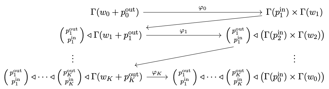
and by the universal property defining $\left[\begin{smallmatrix}-\\-\end{smallmatrix}\right]$, this is equivalent to the desired map. So in the case of (rnWD2), this would be All together these give rise to a map $$E\mathcal{y}^E\otimes AB\mathcal{y}^{ACE}\to AE\mathcal{y}^{CD}\triangleleft DB'\mathcal{y}^E$$ as desired.

5 Conclusion

In this post we showed how recumbent wiring diagrams provide a syntax for $\mathbb{O}\mathbf{rg}_\mathfrak{m}$ by specifying a functor $$\mathit{MP}\colon\mathbf{rnWD}\to\mathbb{O}\mathbf{rg}_\mathfrak{m}$$ from a cyclic operad of wiring diagrams into this complicated object $\mathbb{O}\mathbf{rg}_\mathfrak{m}$. Both the objects and the morphisms in $\mathbb{O}\mathbf{rg}_\mathfrak{m}$ are much more general than what arise from the functor. But $\mathit{MP}$ gives a baseline understanding of what is possible in $\mathbb{O}\mathbf{rg}_\mathfrak{m}$. While maps in $\mathbb{O}\mathbf{rg}_\mathfrak{m}$ might be called “evolving planners" or”evolving programs”, some of these are given by pure message passing, or pure “neuron firing” protocols, as dictated by a neural wiring diagram.

Footnotes

1. It turns out that the free monad monad $\mathfrak{m}$ is monoidal as a functor, but not as a monad, with respect to the $\vee$-product; in particular, the monad multiplication is not a $\vee$-monoidal natural transformation. This means that the Kleisli category of the free monad monad is not monoidal, but only pre-monoidal, with respect to $\vee$. This post only relies on the $+$-monoidal structure, and every monad is monoidal with respect to coproducts when they exist. Hence, this post still stands. I will make appropriate edits throughout.

2. See the edit at the top of this blog post.