A dynamic monoidal category for strategic games

Abstract

After last month’s wonderful ACT conference at University of Strathclyde in Glasgow, David Spivak and I spent some time with Matteo Capucci and Riu Rodriguez Sakamoto talking about how our theory of dynamic monoidal categories can model the non-cooperative strategic games that they study at Strathclyde. A dynamic monoidal category is an elegant way to formalize a version of compositional game theory based on Matteo’s work in, where games can be composed both sequentially and in parallel with the players updating their strategies by applying “counterfactual reasoning” to their payoffs in a functorial way.

After July’s wonderful ACT conference at University of Strathclyde in Glasgow, David Spivak and I spent some time with Matteo Capucci and Riu Rodriguez Sakamoto talking about how our theory of dynamic monoidal categories (Shapiro, Brandon T. and Spivak, David I. 2022) can model the non-cooperative strategic games that they study at Strathclyde. A dynamic monoidal category is an elegant way to formalize a version of compositional game theory based on Matteo’s work in (Capucci 2022), where games can be composed both sequentially and in parallel with the players updating their strategies by applying “counterfactual reasoning” to their payoffs in a functorial way.

1 Strategic games

We will take as our “interfaces” pairs of sets (A,A'), where A is regarded as the possible positions at one point in a game and A' consists of the potential payoffs. Making a play (or in a multi-turn game, a move) between two interfaces (A,A') and (B,B') amounts to choosing for a given position in A a new position in B, as well as how to interpret a payoff of the new position (from B') into a payoff of the original position (in A'). I interpret this backwards map on payoffs as encoding that the payoff comes from the new position in B but the player makes decisions from the vantage point of the original position in A, so the payoff of a move needs to be interpreted into A'.

So a “game” is then just a pair of interfaces, which is played by turning a position of the first into a position of the second and interpreting back the payoff. One way a “player” (which will become a technical term later on) could play such a game is with a “strategy” that determines for each position I \in A both a new position in B and a payoff interpretation function B' \to A'.

The aspect of game theory we are looking to model is the dynamics of strategies: when a player plays with a given strategy and sees the results, they may update their strategy, especially if they can analyze what would have happened had they played differently. This is called “counterfactual reasoning” and we can model it as an adjustment to the interfaces by replacing (A,A') with (A,A'^A). So instead of interpreting just the payoff of the play that was made, a player can also see what the payoff would have been for all of the other plays they could have made.

2 Valuation and distribution monads for nondeterminism

The basic idea of a strategic game theory model is to encode how a player changes their strategy based on additional information as it becomes available. A strategy can be regarded as a state in an open dynamical system, where each move and payoff provides new information to inform an updated strategy. Generally, a player will switch to what seems like the best possible strategy, but in practice there may be many equally good strategies without a clear way to choose between them.

In a real life game one of these best strategies might be chosen at random, and we could encode this by changing the states of our system from strategies to probability distributions on the set S of strategies. We could also make our states subsets of S, so that an updated state includes all of the equally optimal strategies. Or perhaps “valuations” on S, which are functions from S to a set of values like \mathbb{R} or [0,1]. In fact, a subset of S is also a kind of valuation where the values belong to the set of booleans \mathbb{B}= \{\bot,\top\} and the function S \to \mathbb{B} sends only the elements in the subset to \top.

Rather than making a fixed choice of how to encode this nondeterminism, we can instead describe a large class of examples and focus on only the properties that they need to satisfy to effectively model strategic game theory. Finitely supported probability distributions generalize using a formalism based on valuations that also describes nonempty subsets, so we will focus on this general class of distributions instead.

Let V be a semiring, which consists of two monoid structures (0,+) and (1,\times) on the same set V satisfying distributivity of \times over +. There is a monad V^{(-)} on \textbf{Set} defined by:

• V^S is the set of finitely supported valuations of S in V (functions V \to S);
• For a function f : S \to T, v : S \to V, and t \in T, define V^f(v) = \sum_{s \in f^{-1}(t)} v(s); \tag{1}
• \eta : S \to V^S sends s \in S to the valuation sending s to 1 and everything else to 0;
• To define \mu : V^{V^S} \to V^S, for s \in S we set \mu(w)(s) = \sum_{v \in V^S} w(v) \times v(s). \tag{2}

The functoriality, naturality, unitality, and associativity equations that make this data form a monad are all guaranteed by the units, associativity, and distributivity of the semiring V. If V admits infinitary sums which \times also distributes over, then a similar monad can be defined sending a set S to the set of all valuations without the assumption of finite support.

For any semiring V there is also a submonad \mathsf{Dist}_V \hookrightarrow V^{(-)}, where \mathsf{Dist}_V(S) consists of the valuations v \in V^S with \sum\limits_{s \in S} v(s) = 1, which are called distributions. When V has multiplicative inverses, there is *almost* a map of monads V^{(-)} \to \mathsf{Dist}_V sending each valuation to its normalization given by scaling according to the inverse of \sum_s v(s). This map is obstructed by valuations which are constant at 0, though it can be defined on the submonad of V^{(-)} containing valuations with nonempty support.

For the semiring (\mathbb{R},0,+,1,\times), \mathbb{R}^{(-)} is the free real vector space monad, and more generally algebras for any valuation monad V^{(-)} are V-modules. Here distributions are precisely finitely supported probability distributions.

We could also consider the semiring (\mathbb{R}_{\ge 0},0,\max,1,\times), which restricts the previous example to the non-negative reals and replaces sums with maxima. In game theory, this has the effect of prioritizing strategies with the best possible value among many possibilities rather than the sum of all its possible values (a more cynical player could also take the minimum, though that would not as easily fit this framework as \min lacks a unit in \mathbb{R}_{\ge 0}). Distributions in this setting are simply valuations whose values do not exceed 1.

For the semiring (\mathbb{B},\bot,\vee,\top,\wedge) of booleans (which does have infinite sums), \mathbb{B}^{(-)} is the powerset monad. In this case Equation (1) unwinds to the direct image of a subset, the unit sends each element of S to the corresponding singleton subset, and Equation (2) unwinds to the union of a subset of subsets. Here a distribution is any nonempty subset.

When playing a game and deciding which strategy to choose, a valuation is only as useful as its associated distribution when it has one, as both encode equally well the information of which strategy is the best. However, distributions or at least normalizable valuations are preferable, as a valuation sending every strategy to zero would make it very difficult to decide how to play.

A convenient property of a valuation monad V^{(-)} is that it sends coproducts to products when V has infinitary sums, meaning in particular that V^S \cong \prod_{s \in S} V^{\{s\}}. When V has only finite sums, V^S is the subset of the corresponding product containing tuples with finite support. This property, in either form, is not shared by the distribution monad, which sends the singleton set to itself. However, when V admits normalization there is a natural map \mathrm{norm} : \left(\prod_{s \in S} V^{\{s\}}\right) \backslash \mathop{\mathrm{const}}_0 \cong V^S \backslash \mathop{\mathrm{const}}_0 \to \mathsf{Dist}_V(S), which we will use to update a player’s distribution on a set of strategies.

3 Dynamic monoidal categories

The main idea of modeling game theory as a dynamic monoidal category is that distributions on the set of strategies can be regarded as morphisms which can be updated, tensored, and composed (corresponding to the “dynamic,” “monoidal,” and “category” structure respectively). Dynamic monoidal categories were defined in (Shapiro, Brandon T. and Spivak, David I. 2022 Definition 3.7), and combine the structure of a monoidal category with that of polynomial coalgebras on the hom-sets.

For a polynomial p, a p-coalgebra is a set X of states equipped with an “action” function \textnormal{act}: X \to p(1) and, for each x \in X, an “update” function \textnormal{upd}_x : p[\textnormal{act}(x)] \to X. The set X can then be treated as the states of an open dynamical system, where each state x is labeled by some position in p(1) and when given a direction updates to \textnormal{upd}_x applied to that direction.

A relaxed dynamic monoidal category {\textbf{A}} consists of:

• a monoid ({\textbf{A}}_0,e,*) of objects;
• for each a \in {\textbf{A}}_0, a polynomial p_a;
• an isomorphism of polynomials y \cong p_e;
• for each a,a' \in {\textbf{A}}_0, a “laxator” morphism of polynomials p_{a} \otimes p_{a'} \to p_{a*a'} (this is a slight generalization of (Shapiro, Brandon T. and Spivak, David I. 2022), where this map is an isomorphism);
• for each a,b \in {\textbf{A}}_0, a [p_a,p_b]-coalgebra {\textbf{X}}_{a,b};
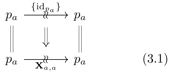
• for each a \in {\textbf{A}}_0, an “identitor” morphism of coalgebras as in Equation (3.1);
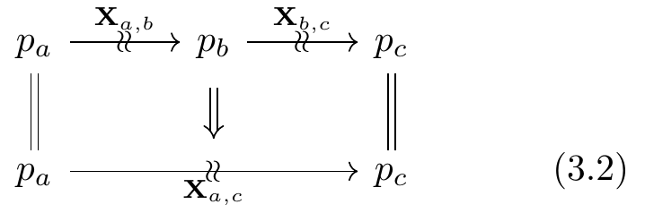
• for each a,b,c \in {\textbf{A}}_0, a “compositor” morphism of coalgebras as in Equation (3.2); and
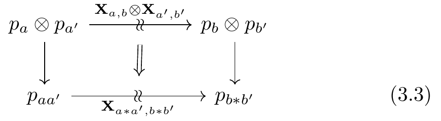
• for each a,a',b,b' \in {\textbf{A}}_0, a “productor” morphism of coalgebras as in Equation (3.3):

satisfying unit, associativity, and interchange equations.

In the dynamic monoidal category for strategic games, the monoid of objects will be pairs of sets (A,A') with pairwise product as the monoid structure. We can regard an interface (A,A') as a polynomial p_{A,A'} = A\mathcal{y}^{A'}, where a morphism of polynomials A\mathcal{y}^{A'} \to B\mathcal{y}^{B'} is the same as a strategy from the interface (A,A') to (B,B'): it consists of functions A \to B and A \times B' \to A' (also called a lens). While we will only consider monomials, counterfactual reasoning can be modeled as a more general construction on \textbf{Poly}.

For any polynomial p, let p^\square = p(1)\mathcal{y}^{\Gamma(p)}, where \Gamma(p) is the set of sections of p, or rather, choices of i \in p[I] for all I \in p(1). The polynomial associated to (A,A') in our relaxed dynamic monoidal category will be p_{(A,A')}^\square = A\mathcal{y}^{A'^A}, where this construction can be thought of as a “counterfactual replacement” of a polynomial, whose directions encode not just the payoff of a position in p but also payoffs for all of the other possible positions.

The assignment p \mapsto p^\square is an endofunctor on \textbf{Poly}, and there is a natural transformation p \to p^\square which is the identity on p(1) and on directions sends (I \in p(1),\gamma \in \Gamma(p) to \gamma(I) \in p[I]. It is also a lax monoidal functor with respect to the Dirichlet tensor product \otimes on \textbf{Poly}, where y^\square \cong y and the morphism p^\square \otimes q^\square \to (p \otimes q)^\square is again the identity on the positions p(1) \times q(1); on directions it sends ((I,J) \in p(1) \times q(1), \gamma \in \Gamma(p \otimes q)) to the pair (\gamma_p,\gamma_q) \in \Gamma(p) \times \Gamma(q), where \gamma_p(I') = \gamma(I',J) and \gamma_q(J') = \gamma(I,J'). Matteo calls this map of polynomials the “Nashator,” as it picks out each row and column in a payoff matrix of possible plays by two players in a game, similar to the matrices in which Nash equilibria are found. This map will serve as the laxator in our relaxed dynamic monoidal category, where the modifier “relaxed” refers to the fact that the Nashator is not an isomorphism.

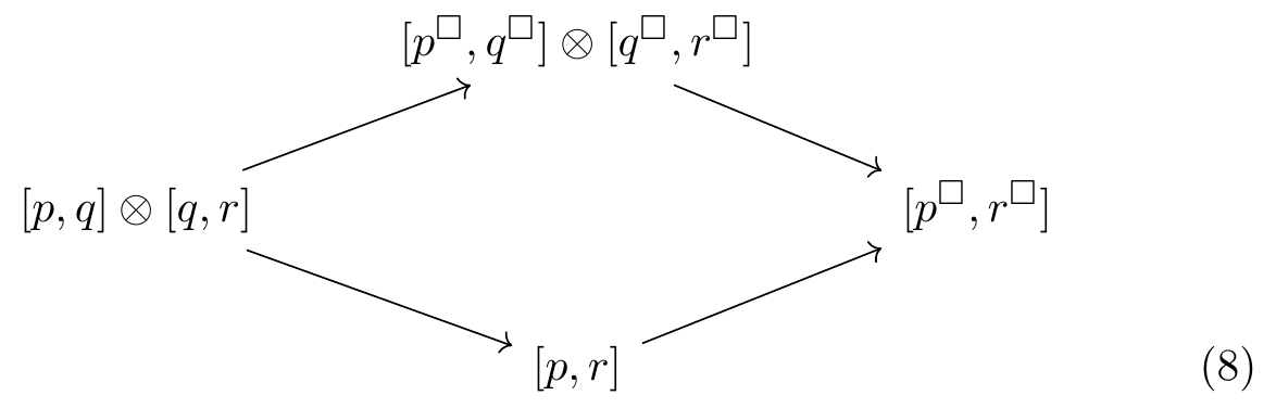
From this structure alone we can show how (-)^\square interacts with the monoidal closed structure of \otimes. Recall that [p,q] = \sum_{f : p \to q} \mathcal{y}^{\sum_{I \in p(1)} q[fI]} is the internal hom polynomial equipped with an evaluation map p \otimes [p,q] \to q. This lets us define a map p^\square \otimes [p,q]^\square \to \left( p \otimes [p,q] \right)^\square \to q^\square. Using the universal property of the closure and the natural transformation \mathrm{id}_\textbf{Poly}\to (-)^\square, we then get a map of polynomials [p,q] \to [p,q]^\square \to [p^\square,q^\square], which will facilitate modeling the behavior of players in this structure. On positions, this map sends a map f : p \to q to f^\square : p^\square \to q^\square, which acts the same as f on positions and on directions sends (I \in p(1),\gamma_q \in \Gamma(q)) to \gamma_p \in \Gamma(p) where \gamma_p(I') = f^\#(\gamma_q(f(I'))).

4 Players and information as coalgebra states

We can now properly define what a player is in this model: a game is played between interfaces (A,A') and (B,B'), and a player consists of a set S and a polynomial morphism \phi : \mathsf{Dist}_V(S)\mathcal{y}^V \to [A\mathcal{y}^{A'},B\mathcal{y}^{B'}] for some fixed distribution monad \mathsf{Dist}_V. The set S consists of abstract strategies, which have names but are not yet realized as polynomial morphisms A\mathcal{y}^{A'} \to B\mathcal{y}^{B'}. The morphism \phi on positions describes how the player takes a distribution on all of their possible abstract strategies and converts it to a concrete strategy. On directions, \phi accounts for the value the player receives when applying their concrete strategy to a given position in A and payoff from B'.

To simplify the notation, we will use p and q to refer to both the pairs (A,A') and (B,B') as well as their canonical polynomials. The [p^\square,q^\square]-coalgebra {\textbf{X}}_{p,q} of arrows from p to q in our dynamic monoidal category has states which consist of a player and a distribution on their strategy set, representing their current assessment of the possible strategies based on available information. Formally, the state set is defined as X_{p,q} = \left\{(S,\phi,v) \;\;\middle|\;\; S : \textbf{Set}, \;\; \phi : \mathsf{Dist}_V(S)\mathcal{y}^V \to [p,q], \;\; v \in \mathsf{Dist}_V(S) \right\}. The action X_{p,q} \to [p^\square,q^\square](1) sends (S,\phi,v) to \phi(v)^\square : p^\square \to q^\square, and the update of (S,\phi,v) sends (I \in p(1),\gamma \in \Gamma(q)) to \left(S,\phi, \mathop{\mathrm{norm}}\left(s \mapsto \phi^\#(I,\gamma(\phi(\eta s)(I)))\right) \right). \tag{4} This normalization requires that \phi^\# sends some pair (I,\gamma(\phi(\eta s))) to a nonzero value, which we will assume throughout.

Here \eta s is the distribution sending s to 1 and all other abstract strategies in S to 0, so the update formula in Equation (4) uses counterfactual reasoning by checking what value (according to \phi^\#) would have been achieved by employing with certainty the strategy s on the same position a. The section \gamma provides the counterfactual of what payoff would have been received from the move \phi(\eta s)(I), and \phi^\# encodes how to extract a value from that counterfactual to build a new distribution. While we use the general polynomial notation of p and q, it is essential that q = B\mathcal{y}^{B'} (rather than a more general polynomial) so that the potential payoffs for different moves are of the same type and hence (I,\gamma(\phi(\eta s)(I))) is in fact a well-typed direction of [p,q].

Like many dynamic structures, the states of this coalgebra consist of some fixed information (the player (S,\phi)) which does not get updated, as well as an updating parameter (here the distribution v). However, the algebraic structure of a dynamic monoidal category describes primarily how players can be combined in series or parallel.

5 Identity games

The simplest piece of the monoidal category structure on these dynamical systems is the identitors, which amount to a state in each X_{p,p} that is left fixed by updates. This state is given by (1, \mathop{\mathrm{const}}_\mathrm{id}: \mathcal{y}^V \to [p,p], * \in \mathsf{Dist}_V(1) \cong 1), where \mathop{\mathrm{const}}_\mathrm{id} sends the unique position in \mathcal{y}^V to \mathrm{id}_p on positions and on directions sends each (a,b) to 1. As \mathsf{Dist}_V(1) \cong 1, the update function always outputs the same state.

Game theoretically, this state describes a player who always keeps the current position and values all payoffs equally.

6 Parallel games

The productor consists of a function X_{p,q} \times X_{p',q'} \to X_{p \otimes p',q \otimes q'} on states which respects actions and updates, and describes how to treat two players in parallel games as a single player playing two parallel games at once. This function sends (S,\phi,v) and (S',\phi',v') to (S \times S',\phi \star \phi', v \times v'), where v \times v' sends (s,s') to v(s)v'(s') and \begin{aligned} \phi \star \phi' : \mathsf{Dist}_V(S \times S')\mathcal{y}^V &\to \mathsf{Dist}_V(S)\mathcal{y}^V \otimes \mathsf{Dist}_V(S')\mathcal{y}^V \\&\to [p,q] \otimes [p',q'] \\&\to [p \otimes p',q \otimes q']. \end{aligned} \tag{5}

The first map in Equation (5) is defined on positions by (\mathsf{Dist}_V(\pi_1),\mathsf{Dist}_V(\pi_2)) : \mathsf{Dist}_V(S \times S') \to \mathsf{Dist}_V(S) \times \mathsf{Dist}_V(S') and on directions by the semiring multiplication V \times V \to V. More specifically, on positions this map takes a distribution on S \times S' and for each s \in S sums up in V the values of (s,s') for all s' \in S. This means that given a distribution on all pairs of strategies the two players could use in each game, each player evaluates their own strategies accounting for all possible strategies that the other player could choose, and the value of a pair of strategies is given by the sum in V of their separate values.

This has different meanings for different choices of the distribution monad. When V is \mathbb{R} with addition and multiplication, the value of a strategy s \in S is given by adding up the values of all pairs (s,s'), essentially treating all possible strategies of the other player as equally likely to be played. When V is the semiring \mathbb{R}_{\ge 0} and the sum is a maximum, the value of s is determined by its pairing with the best possible choice of s'. In this case the player seems to assume that their collaborator wants what is best for them, while a semiring in which sums are minima would model a more adversarial relationship. Ultimately though, while the productor must specify a map of polynomials from \mathsf{Dist}_V(S \times S')\mathcal{y}^V, we are only concerned with its application to distributions of the form v \times v', as the productor must be a coalgebra map meaning these distributions are closed under updates.

The proof that this function on states preserves actions has essentially two components:

• applying (\mathsf{Dist}_V(\pi_1),\mathsf{Dist}_V(\pi_2)) to the distribution v \times v' yields the pair \left(\sum_{s' \in S'} v'(s')\right)v = v \qquad \textrm{and} \qquad \left(\sum_{s \in S} v(s)\right)v' = v'; and
• the diagram (6) commutes.

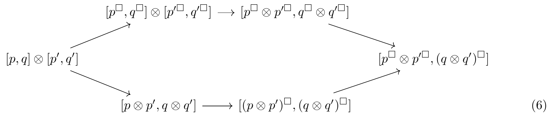
On the other hand, given this it is easy to see that updates are preserved: the morphism [p,q] \otimes [p',q'] \to [p \otimes p',q \otimes q'] is cartesian, so updates as defined in Equation (4) are computed independently and then multiplied together, just as desired.

7 Sequential games

The compositor is defined very similarly to the productor, describing two players making moves one after another rather than in parallel. The function on states X_{p,q} \times X_{q,r} \to X_{p,r} sends (S,\phi,v) and (T,\psi,w) to (S \times T, \;\phi;\psi, \;v \times w), where \begin{aligned} \phi;\psi : \mathsf{Dist}_V(S \times T)\mathcal{y}^V &\to \mathsf{Dist}_V(S)\mathcal{y}^V \otimes \mathsf{Dist}_V(T)\mathcal{y}^V \\&\to [p,q] \otimes [q,r] \\&\to [p,r] \end{aligned} \tag{7} and the first map in Equation (7) is the same as that in Equation (5). Much like the productor describing two strategies running in parallel, the compositor extracts in the same way two concrete strategies and then composes them into one. This is a coalgebra map for the same reasons as the productor, with the commuting diagram (6) replaced by (8).

To complete the definition of this relaxed dynamic monoidal category of interfaces, players, and distributions, we note that the identitors, productors, and compositors satisfy the relevant unit, associativity, and interchange equations nearly by definition, as both productors and compositors are defined by cartesian products of abstract strategy sets and tensor products of the morphisms of polynomials that make those strategies concrete.

8 Conclusion

Strategic game theory includes paradigms for how players update their strategies using counterfactual reasoning, and how sequences of players can be treated as a single player by composing their games in sequence and/or in parallel. The combination and compatibility of these different structures is precisely captured by the relaxed dynamic monoidal category of interfaces, players, and distributions. Our hope is that the study of these dynamic categorical structures can shed light on game theory and more clearly illuminate its connections to other structured dynamical systems such as deep learning.

References

Capucci, M. 2022. “Diegetic Representation of Feedback in Open Games.” Applied Category Theory 2022. 2022. https://msp.cis.strath.ac.uk/act2022/slides/ACT2022_slides_1399.pdf.

Shapiro, Brandon T. and Spivak, David I. 2022. “Dynamic categories, dynamic operads: From deep learning to prediction markets.” https://arxiv.org/abs/2205.03906.