Lenses are semi-monads, maybe lenses are monads
Have you ever heard of a semi-monad? I hadn’t, but when I came across a “monad without unit” in the wild, I made an analogy with semigroups (a semigroup is a group without unit). It seems others have also thought to use the term semi-monad for such a gadget. There is a semi-monad structure on the full subcategory of lenses inside Poly, and this is useful for building logic circuits and other interconnected dynamical systems. In particular, it allows us to formalize what I think is really pretty notation for “speeding up” boxes in wiring diagrams. But what does this mean mathematically? We’ll explain in this post.
1 Introduction
Have you ever heard of a semi-monad? I hadn’t, but when I came across a “monad without unit” in the wild, I made an analogy with semigroups (a semigroup is a group without unit). It seems others have also thought to use the term semi-monad for such a gadget.
Anyway, here’s how it came up for me. Recall that the full subcategory \mathbf{Lens}\subseteq\mathbf{Poly} has objects which we notate by \left[\begin{smallmatrix}{\vphantom{f}A} \\ {\vphantom{f}B} \end{smallmatrix}\right], for any sets A,B. Considered as a polynomial it is the monomial \left[\begin{smallmatrix}{\vphantom{f}A} \\ {\vphantom{f}B} \end{smallmatrix}\right]=B\mathcal{y}^A. I realized that each such object carries an associative multiplication map \mu\colon \begin{bmatrix}{\vphantom{f_f^f}A} \\ {\vphantom{f_f^f}B} \end{bmatrix} \mathbin{\triangleleft} \begin{bmatrix}{\vphantom{f_f^f}A} \\ {\vphantom{f_f^f}B} \end{bmatrix} \to \begin{bmatrix}{\vphantom{f_f^f}A} \\ {\vphantom{f_f^f}B} \end{bmatrix} that works by “outputting the first B and repeating the A”; I’ll explain better below. But there is no corresponding unit; indeed, when B=0 there is no map \mathcal{y}\to B\mathcal{y}^A at all. We can thus call the pair (B\mathcal{y}^A,\mu) a semi-monad.
Being a semi-monad is a little unusual but not so bad; in particular, for any positive integer N\in\mathbb{N}_{\geq1}, there is a well-defined map \mu^N\colon \begin{bmatrix}{\vphantom{f_f^f}A} \\ {\vphantom{f_f^f}B} \end{bmatrix}^{\mathbin{\triangleleft}N}\to \begin{bmatrix}{\vphantom{f_f^f}A} \\ {\vphantom{f_f^f}B} \end{bmatrix} which again is given by “outputting the first B and repeating the A”, as we’ll explain. For now let me say two things about this semi-monad (B\mathcal{y}^A,\mu).
First, if you want, you can simply add \mathcal{y} to the carrier to get \mathcal{y}+B\mathcal{y}^A and, using the inclusion \eta\colon\mathcal{y}\to\mathcal{y}+B\mathcal{y}^A as the unit, you get a full-fledged monad (\mathcal{y}+B\mathcal{y}^A,\eta,\mu). In fact, not only does this extend to a functor (\mathcal{y}+)\colon\mathbf{Lens}\to\mathbf{PolyMnd}, but this functor is fully faithful!
Second, I find the semi-monad structure on B\mathcal{y}^A useful for building logic circuits and other interconnected dynamical systems in \mathbf{Poly}. In particular, it allows us to formalize what I think is really pretty notation for “speeding up” boxes in wiring diagrams.
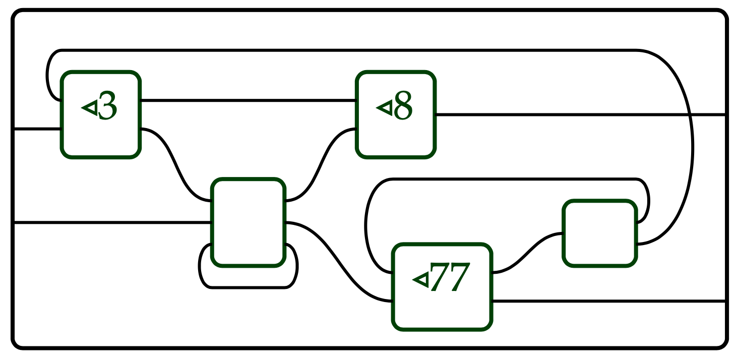
This picture is syntax saying that the outer circuit is run by speeding up whatever’s in the indicated boxes by the indicated factors: they run 3, 8, and 77 times in the time it takes the other boxes to run one clock-tick. But what does it mean mathematically? We’ll explain in this post.
2 The multiplication map
For any A,B\in\mathbf{Set} and positive integer N\in\mathbb{N}_{\geq1}, let’s give a map \mu^N\colon (B\mathcal{y}^A)^{\mathbin{\triangleleft}N}\to B\mathcal{y}^A. Recall that a position of the polynomial (B\mathcal{y}^A)^{\mathbin{\triangleleft}N} is an A-branching B-tree t of height N: every node of t is labeled by an element of B, and there are A-many branches coming out of it. For example, here’s an element of (B\mathcal{y}^A)^{\mathbin{\triangleleft}3}, where A=\{L,R\} and B=\{b_1,b_2,b_3\}:
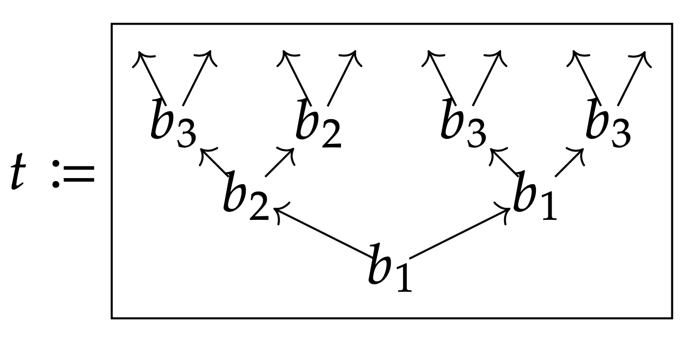
So this tree t is one position of (B\mathcal{y}^A)^{\mathbin{\triangleleft}3}, and its directions set consists of the A^3-many leaves.
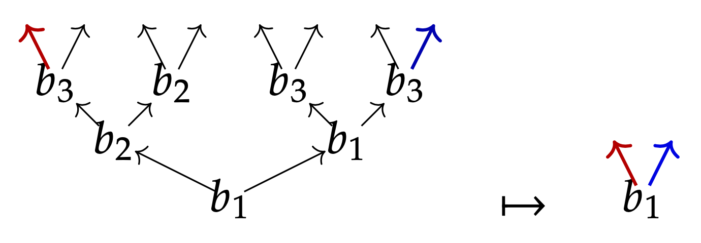
The multiplication map \mu^N, on positions, sends tree t to its root, t\mapsto t.\texttt{root}\in B. On directions, it sends a\in A back to the leaf obtained by choosing the a^{\text{th}} branch all the way up the tree.
3 What this means for dynamical systems
What a map \mu^N\colon (B\mathcal{y}^A)^{\mathbin{\triangleleft}N}\to B\mathcal{y}^A means for dynamical systems is that a machine with inputs A and outputs B, running at the usual speed, can be an interface for a machine with the same inputs and outputs, but running at N-times the speed. It works as follows. Take the first output of the fast machine and present it as the output of the slow machine. Then take any input to the slow machine, and run the fast machine with that input N-many times in a row.
So to the outside world, at each time step, the machine is just giving a single output and accepting a single input. But inside, the machine is running that same input N times in a row, but only outputting one value during that whole time.
Why is this useful? To start with, note that for any function f\colon A\to B, there is an associated (A,B)-machine with state set A, namely A\mathcal{y}^A\to B\mathcal{y}^A given by a\mapsto (f(a), a'\mapsto a'). In other words, if the machine starts in some state a, it first outputs f(a); then it inputs a new a' and updates the state to be a'. Let’s call this the memoryless machine associated to f.
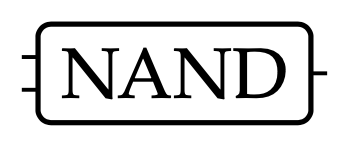
So for example, we can take the function \operatorname{NAND}\colon2\times 2\to 2 that sends a pair (b_1,b_2) of booleans to the boolean \neg(b_1\wedge b_2), and turn it into the memoryless machine
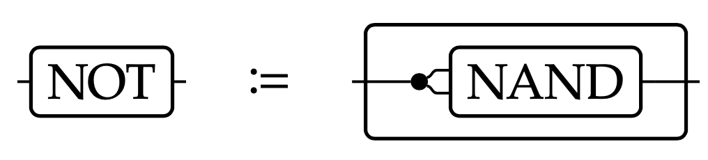
Here’s where the semi-monad structure becomes useful. It is well-known that every logic gate (NOT, AND, OR, etc.), as well as adder circuits, etc., can all be constructed out of NANDs, e.g. the NOT gate is given by \neg(b)=\operatorname{NAND}(b,b), or in wiring diagrams:
But there’s a problem. Suppose we construct \operatorname{OR} in the usual way out of \operatorname{NAND} gates:
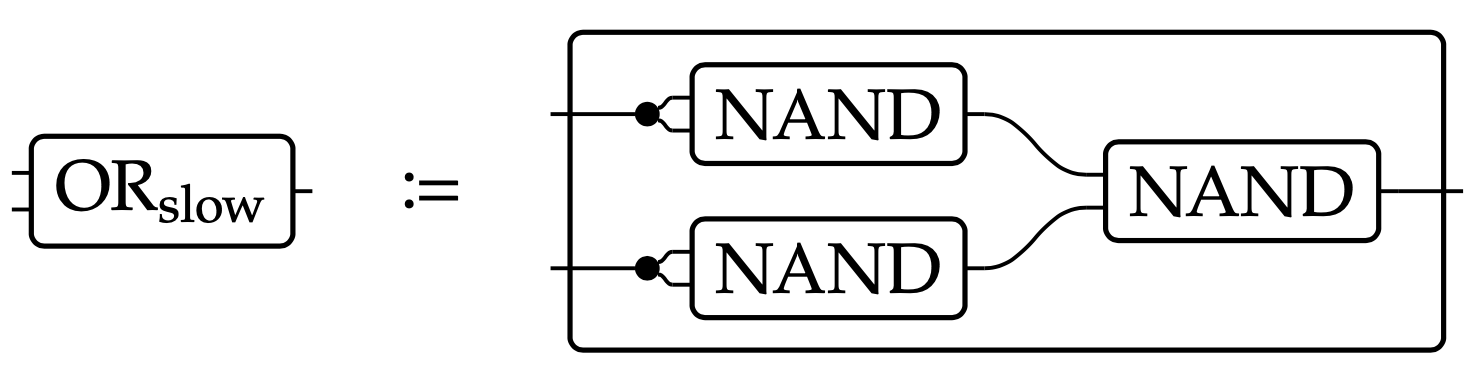
We called it “\operatorname{OR}_\text{slow}” because it’s not the same thing as the memoryless machine associated to \operatorname{OR}\colon 2\times 2\to 2! Indeed, the above circuit takes two clock-ticks for the input to propagate to the output. This can be confusing to someone expecting the memoryless machine \operatorname{OR}.
It is convenient to be able to look at an \operatorname{OR}-box and think of it as a memoryless system. To do so, we should define

This machine has the correct behavior, namely that of the memoryless machine associated to \operatorname{OR}. We can do the same sort of thing to any directed acyclic graph of memoryless machines, e.g. adder circuits: we can run it fast enough to simulate the desired output in a single step.
4 A more technical look
Now let’s say what’s going on here mathematically. Recall that a polynomial comonad (c,\epsilon,\delta) consists of a polynomial c and maps \epsilon\colon c\to \mathcal{y} and \delta\colon c\to c\mathbin{\triangleleft}c, respectively called counit and comultiplication. An important example for us is c\coloneqq\left[\begin{smallmatrix}{\vphantom{f}S} \\ {\vphantom{f}S} \end{smallmatrix}\right]=S\mathcal{y}^S, because a map S\mathcal{y}^S\to p can be identified with a map S\to p\mathbin{\triangleleft}S, i.e. a p-coalgebra with states S. When p=B\mathcal{y}^A, the data of a map S\mathcal{y}^S\to B\mathcal{y}^A is called a Moore machine with inputs A, outputs B, and states S. We often just call it a dynamical system.
So now consider what happens if p=m carries a semi-monad structure (m,\mu), e.g. when m=B\mathcal{y}^A. In this case, if \varphi\colon c\to m is a polynomial map, then for any N\geq 1, we are interested in the composite: c \xrightarrow{\delta^N}c^{\mathbin{\triangleleft}N} \xrightarrow{\varphi^{\mathbin{\triangleleft}N}}m^{\mathbin{\triangleleft}N} \xrightarrow{\mu^N}m It runs the machine N-times in a single time step.
The ability to form the above composite map gives us an action of the multiplicative monoid (\mathbb{N}_{\geq 1},1,\times) of positive integers on the set \mathbf{Poly}(c,m). That is, any positive integer N sends \varphi\in\mathbf{Poly}(c,m) to (\delta^N\mathbin{;}\varphi^{\mathbin{\triangleleft}N}\mathbin{;}\mu^N)\in\mathbf{Poly}(c,m).
Suppose given a wiring diagram \varphi\colon m_1\otimes\cdots\otimes m_k\to m. If all the m_i carry semi-monads, then for any choice of positive integer N_i\geq 1 for each 1\leq i\leq k, we obtain a map m_1^{\mathbin{\triangleleft}N_1}\otimes\cdots\otimes m_k^{\mathbin{\triangleleft}N_k} \xrightarrow{\mu^{N_1}\otimes\cdots\otimes\mu^{N_k}}m_1\otimes\cdots\otimes m_k \xrightarrow{\varphi} m This is the math behind the diagram in Figure 1.
5 The functor \mathbf{Lens}\to\mathbf{PolySemiMnd}
We should also say that equipping a lens \left[\begin{smallmatrix}{\vphantom{f}A} \\ {\vphantom{f}B} \end{smallmatrix}\right] with the semi-monad structure above is functorial. Recall that a map in \mathbf{Lens} of the form \left[\begin{smallmatrix}{\vphantom{f}A} \\ {\vphantom{f}B} \end{smallmatrix}\right]\to\left[\begin{smallmatrix}{\vphantom{f}A'} \\ {\vphantom{f}B'} \end{smallmatrix}\right] is the same thing as a polynomial map \varphi\colon B\mathcal{y}^A\to B'\mathcal{y}^{A'}. So the functoriality says that any such map commutes with the multiplication, in the sense that the following diagram commutes \begin{CD} (B\mathcal{y}^A)^{\mathbin{\triangleleft}N} @>{\varphi^{\mathbin{\triangleleft}N}}>> (B'\mathcal{y}^{A'})^{\mathbin{\triangleleft}N} \\@V{\mu^N}VV @VV{\mu^N}V \\B\mathcal{y}^A @>>{\varphi}> B'\mathcal{y}^{A'} \end{CD} for any N\geq 1. If you want to think through why that is, think about how to convert A-branching B-trees into A'-branching B'-trees via repeated application of \varphi. Now check that this process commutes with taking roots and repeatedly following branches, i.e. it commutes with \mu^N.
In fact, if you’ve done the work to see that \mathbf{Lens}\to\mathbf{PolySemiMnd} is functorial, from there it is relatively easy to check that this functor is fully faithful.
6 Maybe monad on \mathbf{Poly} sends \mathbf{Lens}\to\mathbf{PolyMnd}
If you still feel like semi-monads are weird or suspect, note that you can also turn \left[\begin{smallmatrix}{\vphantom{f}A} \\ {\vphantom{f}B} \end{smallmatrix}\right]\in\mathbf{Lens} into a full-fledged polynomial monad, simply by adding \mathcal{y}. Indeed, there is a monad on \mathbf{Poly} itself which we will call \texttt{maybe}=(\mathcal{y}+): \begin{aligned} \texttt{maybe}\colon\mathbf{Poly}&\to\mathbf{Poly}\\ p&\mapsto\mathcal{y}+p \end{aligned} This is a monad because there’s a unit map p\to \mathcal{y}+p and a multiplication map \mathcal{y}+\mathcal{y}+p\to\mathcal{y}+p satisfying the usual laws.
What’s neat is that when we restrict this functor to \mathbf{Lens}\subseteq\mathbf{Poly}, the result is a polynomial monad1 \begin{CD} \mathbf{Lens} @>>> \mathbf{Poly} \\@V{(\mathcal{y}+)}VV @VV{(\mathcal{y}+)}V \\\mathbf{PolyMnd} @>>> \mathbf{Poly} \end{CD} In other words, whereas B\mathcal{y}^A has a natural semi-monad structure, \mathcal{y}+B\mathcal{y}^A has a natural monad structure.
What was surprising to me is that this functor \mathbf{Lens}\to\mathbf{PolyMnd} is also fully faithful. In other words, the only maps of the form \psi\colon\mathcal{y}+B\mathcal{y}^A\to\mathcal{y}+B'\mathcal{y}^{A'} that respect both the unit and the multiplication are exactly the maps \psi=\mathcal{y}+\varphi that come from \mathbf{Lens}!
7 Conclusion
I told my Topos colleagues Evan and Owen about the above ideas, especially my potential “programming” use-case. Evan told me about data flow programming and said that this seemed somewhat similar. But they both warned me that this way of “speeding up” dynamical systems didn’t seem like a good programming paradigm, because you don’t want to always be thinking about the timing of things. This makes me want to clarify my communication a bit more before closing.
First, the semi-monad structure on \left[\begin{smallmatrix}{\vphantom{f}A} \\ {\vphantom{f}B} \end{smallmatrix}\right]=B\mathcal{y}^A just exists and the monad structure on \mathcal{y}+B\mathcal{y}^A also just exists, and it’s pretty neat that they extend to fully faithful functors \mathbf{Lens}\to\mathbf{PolySemiMnd} \qquad\text{and}\qquad \mathbf{Lens}\to\mathbf{PolyMnd} What a mathematician or programmer may find useful about these mathematical facts is up to them.
Second, I am personally interested in the semi-monad structure on \left[\begin{smallmatrix}{\vphantom{f}A} \\ {\vphantom{f}B} \end{smallmatrix}\right] because I had been worried about claiming that you can put together \operatorname{NAND} gates—as dynamical systems—to form other logic gates, given that more complex gates are not memoryless in the same way, i.e. they take more time to run.2 In terms of programming, I was thinking that I’d want to have a kind of virtual “shelf” that holds my favorite dynamical systems. Starting with \operatorname{NAND}, I’d want to build \operatorname{OR} and put that on the shelf, and then adder circuits, etc. But I don’t ever want to think about how long \operatorname{OR} takes; the designer should take care of that for me. So for this shelf idea to work, you should make \operatorname{OR}_\text{slow} out of three \operatorname{NAND} gates, you should indicate mathematically that this circuit takes two clock-ticks to reach equilibrium, hence making \operatorname{OR}\coloneqq(\operatorname{OR}_\text{slow})^{\mathbin{\triangleleft}2}, and then you should put that machine on the shelf. When people take it off the shelf to use later, they don’t have to worry about its timing: in their mind they can think that everything takes one tick to perform its denotative function.
In other words, the semi-monad structure allows us to formalize the “spec sheet”, which says that the circuit needs to be run twice in order to get the expected results, and to embed that information into the \operatorname{OR} object itself.
I’m not sure whether this will be useful in real programming one day. Certainly it’s very low-level programming. It’s interesting to me because I’m fascinated by the possibility that \mathbf{Poly} could be involved throughout computer science, from the very high-level dependent type theories to the very low-level “automata” operations.
Footnotes
Objects in \mathbf{Poly} can be understood as functors \mathbf{Set}\to\mathbf{Set}, so we’re saying that, as a functor, \mathcal{y}+B\mathcal{y}^A is a monad on \mathbf{Set}. So you could say that \mathcal{y}+B\mathcal{y}^A is a \mathbin{\triangleleft}-monoid, or even a monad, in \mathbf{Poly}. We’re also saying that the process of adding \mathcal{y} is itself a monad on \mathbf{Poly}, because it takes polynomials to new polynomials. It just so happens to take monomials (objects in \mathbf{Lens}) to polynomial monads.↩︎
Full disclosure: I’ve known about this solution, using the semi-monad structure on B\mathcal{y}^A, since January 2021. I hadn’t thought about the functoriality, the full-faithfulness, or the monad structure on \mathcal{y}+B\mathcal{y}^A until more recently.↩︎