Spooling out syntax from behavior
polynomial functors
dynamical systems
programming languages
Abstract
The behavior of a dynamical system is its entire fate or character: the tree consisting of precisely what it will do when exposed to any particular sequence of inputs. In the world of polynomial functors, behavior for a dynamical system with interface p is formalized using the cofree comonad \mathfrak{c}_p. On the other hand, syntax in a given language p is formalized using the free monad \mathfrak{m}_p. In this post we explain a sense in which one can extract syntax from behavior: briefly, given a map q\mathbin{\triangleleft}p\to p\mathbin{\triangleleft}q, you get a map \mathfrak{c}_{p\mathbin{\triangleleft} q}\to\mathfrak{c}_p\mathbin{\triangleleft}\mathfrak{m}_q, which we call the associated spooling map. We give a variety of examples, a bit of basic theory, and a program—written entirely as a few arrows of \mathbf{Poly}—for computing conditioned probabilities and expected value of a repeating lottery system.
1 Introduction
In this post, I’ll assume you have some degree of familiarity with polynomial functors. I’ll explain a bit about the cofree comonad \mathfrak{c}_p and the free monad \mathfrak{m}_p on p, and then I’ll discuss some interesting ways in which they are related.
Today we will think of a polynomial p\coloneqq\sum_{I:p(1)}\mathcal{y}^{p[I]} in two ways: as the interface for a dynamical system and as a language.
As an interface, we think of elements I:p(1) as positions that a dynamical system can be in, and for each such position I, we think of p[I] as the set of directions or inputs that it can receive. We imagine that a dynamical system inhabits this interface, by which it interacts with the world. A p-behavior tree T for this interface is a potentially-infinite tree describing precisely what the system will do when exposed to any particular sequence of inputs that it can receive. That is, T consists of a current position and, given any direction it can receive there, another behavior tree. This behavior tree again consists of a current position, and given any direction it can receive there, yet another behavior tree. For example, suppose that p=\{{\color{#057F4C}\bullet}\}\mathcal{y}^2+\{{\color{#0800FF}\bullet},{\color{#FEBD01}\bullet}\}\mathcal{y}+\{{\color{#FE0101}\bullet}\}. It can be in position {\color{#057F4C}\bullet} in which case it could be taken in either of two possible directions, in position {\color{#0800FF}\bullet} or {\color{#FEBD01}\bullet} in which case there is only one direction it can go, or in position {\color{#FE0101}\bullet} in which case it cannot go on. So here are three possible behavior trees:
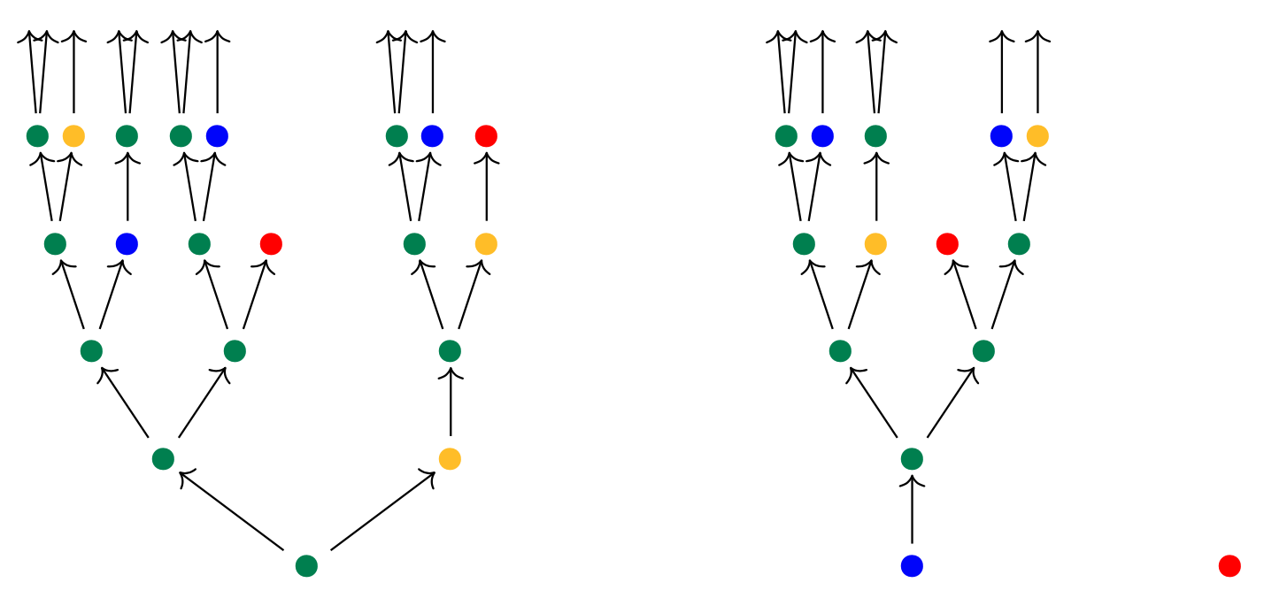
The tree’s root reads out the current position, either a green, blue, yellow, or red dot, and then the tree branches accordingly. All this data—the entire fate of these and any other such tree T—is captured in the cofree comonad \mathfrak{c}_p. It is a polynomial derived from p: its set of positions \mathfrak{c}_p(1) is exactly the set of all p-behavior trees, and its directions at a given tree T is the set of all finite paths starting from the root of T and ending at some node.
But as we said, we can also view p as a language for syntactic formulas. In that case we might think of elements I:p(1) as operations, and each i:p[I] as variables for that operation. For example, suppose p is given by p\coloneqq\{{\color{B20000}+}, {\color{B20000}\times}\}\mathcal{y}^2+\{{\color{B20000}-}\}\mathcal{y}+\{{\color{B20000}0},{\color{B20000}1}\} The operations {\color{B20000}+} and {\color{B20000}\times} each have two variables, the operation {\color{B20000}-} has one variable, and the operations {\color{B20000}0} and {\color{B20000}1} have no variables (they are constants). Then a p-syntax tree T might look as follows:
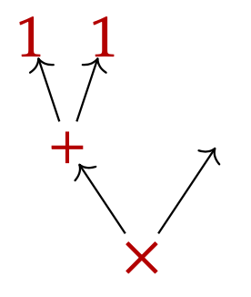
It represents the expression (1+1)\times a for some variable a, which sits at the open leaf on the right. All this data, including all such trees and their open leaves, is captured by the free monad \mathfrak{m}_p. It is a polynomial derived from p: its set of positions is exactly the set of all p-syntax trees, and its directions at a given tree T are all the open leaves of T, i.e. variables in that formula.
So both the cofree comonad \mathfrak{c}_p and the free monad \mathfrak{m}_p have something to do with p-shaped trees. But how are they related mathematically? It turns out there are many interesting relationships.
Back in 2021, David Jaz Myers explained to me that \mathfrak{c}_p(1) always has the structure of a topological space. If each p[I] is finite, it is a profinite space, also known as a boolean algebra, but in general it will be a prodiscrete space. In 2022 June, I gave a Topos seminar talk where I showed that \mathfrak{m}_p gives a basis for the topology on \mathfrak{c}_p.
In 2023 February, I gave another Topos seminar talk where I showed that free monads are modules over cofree comonads. That is, for any polynomials p and q, there is a map1 \Phi_{p,q}\colon\mathfrak{m}_p\otimes\mathfrak{c}_q\to\mathfrak{m}_{p\otimes q}. This map presents \mathfrak{m} as a module over \mathfrak{c}, as described in the nLab.
I find \Phi_{p,q} really useful in that it lets you feed a list of inputs to a dynamical system and receive a list of outputs. Indeed, if p=B\mathcal{y}^A is the interface for an (A,B)-Moore machine, then an element of \mathfrak{c}_{B\mathcal{y}^A} represents a behavior of such a Moore machine, and an element of \mathfrak{m}_{A\mathcal{y}} represents a list of inputs. The composite map \mathfrak{m}_{A\mathcal{y}}\otimes\mathfrak{c}_{B\mathcal{y}^A}\to\mathfrak{m}_{A\mathcal{y}\otimes B\mathcal{y}^A}\to\mathfrak{m}_{B\mathcal{y}} takes a list of A-inputs and an (A,B)-Moore machine and produces the list of B-outputs.
So there are some interesting relationships between cofree comonads and free monads. For the remainder of this blog post, I want to explain yet another interaction between \mathfrak{c} and \mathfrak{m}. Namely, given any polynomials p,q and swap map2 \sigma\colon q\mathbin{\triangleleft}p\to p\mathbin{\triangleleft}q we obtain two spooling maps, which are what this blog post is about: \vec{\sigma}\colon\mathfrak{c}_{p\mathbin{\triangleleft}q}\to\mathfrak{c}_p\mathbin{\triangleleft}\mathfrak{m}_q \qquad\text{and}\qquad \overset{\leftarrow}{\sigma}\colon\mathfrak{c}_{q\mathbin{\triangleleft}p}\to\mathfrak{c}_p\mathbin{\triangleleft}\mathfrak{m}_q. \tag{1} As you can see, you start with some kind of fancy behavior tree, and you read out a simpler behavior tree and a simpler syntax tree, before returning back to the fancy behavior tree. Intuitively, we use the map q\mathbin{\triangleleft}p\to p\mathbin{\triangleleft}q to unwind a sequence (p\mathbin{\triangleleft}q)\mathbin{\triangleleft}\cdots\mathbin{\triangleleft}(p\mathbin{\triangleleft}q) to a sequence (p\mathbin{\triangleleft}\cdots\mathbin{\triangleleft}p)\mathbin{\triangleleft}(q\mathbin{\triangleleft}\cdots\mathbin{\triangleleft}q).
I’ll begin with a few examples to build intuition, then I’ll give a bit of general theory, and then end with some applications for lotteries. Thanks to Owen Lynch for helpful comments on an earlier draft of this post.
2 Examples
Ok, so what’s going on here? What does spooling feel like?
2.0.1 Example 1, log files
For any set A and polynomial p, there is a swap map \sigma\colon A\mathcal{y}\mathbin{\triangleleft}p\to p\mathbin{\triangleleft}A\mathcal{y}. A position in the left-hand side is a pair (a,I) where a:A and I:p(1). It is sent by \sigma to a pair consisting of I:p(1) and the constant function p[I]\to A, which sends each i\mapsto a. It is a bijection on directions. By our general theory (1), \sigma induces a spooling map \vec{\sigma}\colon\mathfrak{c}_{p\mathbin{\triangleleft}A\mathcal{y}}\to\mathfrak{c}_p\mathbin{\triangleleft}\mathfrak{m}_{A\mathcal{y}}. What does it mean? Suppose you have a behavior tree that at each node outputs both a position of p and, for every direction there, an element of A and a remaining tree of the same sort. Then from this, I can extract just the p stuff as its own tree, and if you give me a finite path up that tree, I can tell you all the finite sequence of all the A’s you passed along the way. The map spools out lists of A’s.
2.0.2 Example 2, exceptions
For any polynomial p, there is a distributive law of the maybe monad \mathcal{y}+1 over p: \sigma\colon p\mathbin{\triangleleft}(\mathcal{y}+1)\to(\mathcal{y}+1)\mathbin{\triangleleft}p. It works as follows. Suppose given a position I:p(1) and for every direction i:p[I] we’re given either just a value or an exception. The the map returns an exception if any of the directions do, but otherwise does a no-op, i.e. keep everything the same. By our general theory, \sigma induces a spooling map \vec{\sigma}\colon\mathfrak{c}_{p+1}\to\mathfrak{c}_{\mathcal{y}+1}\mathbin{\triangleleft}\mathfrak{m}_p. This map says that if we have a behavior tree T that at each node either stops or prints a position of p and branches accordingly, then I can extract the amount of time N that it runs without any exceptions: this is either finite or infinite.3 If you give me any amount of time N'\leq N, I can also produce the p-tree up to that point. Since it will only be finite, it will be a syntax tree. For any leaf of that tree, I can return to the behavior tree T, starting at the specified point.
2.0.3 Example 3, sampling
For any polynomial p and natural numbers N_1,N_2:\mathbb{N}, the unitors and associators induce an isomorphism \alpha_{N_1,N_2}\colon p^{\lhd N_1}\mathbin{\triangleleft}p^{\lhd N_2}\xrightarrow{\cong} p^{\lhd N_2}\mathbin{\triangleleft}p^{\lhd N_1}, where p^{\lhd 0}=\mathcal{y} and p^{\lhd N+1}=p\mathbin{\triangleleft}(p^{\lhd N}). Maps of the above form include \alpha_{1,0}\colon p\mathbin{\triangleleft}\mathcal{y}\to\mathcal{y}\mathbin{\triangleleft}p, \alpha_{0,1}\colon \mathcal{y}\mathbin{\triangleleft}p\to p\mathbin{\triangleleft}\mathcal{y}, and the identity \alpha_{1,1}\colon p\mathbin{\triangleleft}p\to p\mathbin{\triangleleft}p. By our general theory, these give rise to maps \vec{\alpha}_{N_1,N_2}\colon\mathfrak{c}_{p^{\lhd N_1+N_2}}\to\mathfrak{c}_{p^{\lhd N_1}}\mathbin{\triangleleft}\mathfrak{m}_{p^{\lhd N_2}}. Note that we can compose this with the map \mathfrak{c}_p\to\mathfrak{c}_{p^{\lhd N_1+N_2}}, which takes a p-tree and returns what looks like the same p-tree, except now chunked up into (N_1+N_2)-sized pieces. So what does the whole map \mathfrak{c}_p\to\mathfrak{c}_{p^{\lhd N_1}}\mathbin{\triangleleft}\mathfrak{m}_{p^{\lhd N_2}} do? Let’s start with N_1=0 and N_1=1, and begin by noting that \mathfrak{c}_\mathcal{y}=\mathcal{y}^\mathbb{N}. The map \mathfrak{c}_p\to\mathfrak{c}_\mathcal{y}\mathbin{\triangleleft}\mathfrak{c}_p takes a p-behavior tree T, asks for a natural number n, produces the height-n syntax tree at the bottom of T, and for any leaf of it, returns the remaining behavior tree. This seems like it could be useful.
Now let’s try N_1=1 and N_2=0, and begin by noting that \mathfrak{m}_\mathcal{y}=\mathbb{N}\mathcal{y}. The map \mathfrak{c}_p\to\mathfrak{c}_p\mathbin{\triangleleft}\mathcal{y} takes a p-behavior tree T, asks for any finite path up it, produces its length, and then (for the unique leaf) returns the remaining behavior tree.
Things start to get interesting with N_1=N_2=1. The map \mathfrak{c}_p\to\mathfrak{c}_p\mathbin{\triangleleft}\mathfrak{m}_p takes a p-behavior tree T, and for any length-n path to some node x, extracts the height-n syntax tree starting at x, and for any leaf of it, returns the remaining behavior tree. We leave the general case (e.g. N_1=3, N_2=5) to the interested reader, who can decide for themselves if “sampling” is a fitting name for this.
2.0.4 Example 4, linearization
For any polynomial p:\mathbf{Poly}_{}, we denote its linearization as \bar{p}\coloneqq p(1)\mathcal{y}; this polynomial has the same positions but a single direction at each. We will be interested in two maps p\to \bar{p}\mathbin{\triangleleft}p \qquad\text{and}\qquad \bar{p}\mathbin{\triangleleft}p\to p\mathbin{\triangleleft}\bar{p}. The first is very simple: it just repeats the position I and is a bijection 1\times p[I]\to p[I] on directions. The second does a swap: it takes (I, I') and returns (I',I), again a bijection on directions. Using these, by our general theory we get \mathfrak{c}_p\to\mathfrak{c}_{p\mathbin{\triangleleft}\bar{p}}\to\mathfrak{c}_p\mathbin{\triangleleft}\mathfrak{m}_{\bar{p}}. This says that if we have a p-behavior tree and you give me any finite path up it, I can return the list of outputs it produced along the way.
2.0.5 Example 5, effects handling
I feel like there should be some story involving both spooling and effects handling, in the sense Owen Lynch and I worked out a few months ago. There, one has a processor polynomial s, whose positions represent states and whose directions represent threads, as well as two other polynomials p,q, and a map \sigma\colon s\mathbin{\triangleleft}q\to p\mathbin{\triangleleft}s \tag{2} And when q=p, we obtain a spooling map \vec{\sigma}\colon\mathfrak{c}_{p\mathbin{\triangleleft}s}\to\mathfrak{c}_p\mathbin{\triangleleft}\mathfrak{m}_s. The setup from (2) also looks a lot like the Turi-Plotkin operational semantics story, so I wonder if there are interesting questions to explore there.
2.0.6 Example 6, counterfactuals
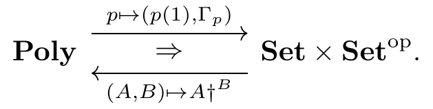
Let \Gamma_p\coloneqq\mathbf{Poly}_{}(p,\mathcal{y}) denote the set of global sections of a polynomial p. This map p\mapsto\Gamma_p, paired with p\mapsto p(1), defines the left adjoint in a distributive monoidal adjunction
We refer to the corresponding lax monoidal monad on \mathbf{Poly}_{} as boxing and denote it \square\colon\mathbf{Poly}_{}\to\mathbf{Poly}_{};4 explicitly, boxing a polynomial p returns the monomial p_\square\coloneqq p(1)\mathcal{y}^{\Gamma_p}. There is also a map p\to p_\square\mathbin{\triangleleft}p_*, where p_*\coloneqq\sum_{I\in p(1)}p[I]\mathcal{y}^{p[I]}, and finally a swap map p_*\mathbin{\triangleleft}p_\square\to p_\square\mathbin{\triangleleft}p_*. Thus we obtain a spooling map \mathfrak{c}_p\to\mathfrak{c}_{p_\square\mathbin{\triangleleft}p_*}\to\mathfrak{c}_{p_\square}\mathbin{\triangleleft}\mathfrak{m}_{p_*}. \tag{3} Note that \mathfrak{c}_{p_\square} is the universal Moore machine for interface p_\square=p(1)\mathcal{y}^{\Gamma_p}. Given a p-behavior tree T, the resulting p_\square-Moore machine M_T:\mathfrak{c}_{p_\square}(1) outputs a position of p, and inputs not just direction of p there but instead a whole suite (i.e. a global section) \gamma:\Gamma_p of directions; these will provide keys for extracting the “counterfactual” information from T. Indeed, if you give me any path through M_T, I can return a p_*-syntax tree that includes all the counterfactual information from T up to that point, as well as the actual path taken in T.
2.0.7 Example 7, coalgebras
A p-coalgebra consists of a set S and a function f\colon S\to p\mathbin{\triangleleft}S, but this is the same as a swap map S\mathbin{\triangleleft}p\to p\mathbin{\triangleleft}S. Hence any coalgebra gives rise to a spooling map \overset{\leftarrow}{f}\colon\mathfrak{c}_S\to\mathfrak{c}_p\mathbin{\triangleleft}\mathfrak{m}_S. Using the unique map \mathfrak{m}_S\to 1, one obtains the usual “anamorphism” function S\to\mathfrak{c}_p\mathbin{\triangleleft}1 from S to the terminal p-coalgebra, induced by f. One way to capture the correctness of \overset{\leftarrow}{f} is in the commutativity of the following diagram: \begin{CD} \begin{bmatrix}\mathfrak{m}_S\\\mathfrak{c}_S\end{bmatrix} @>{\overset{\leftarrow}{f}}>> \mathfrak{c}_p \\@AAA @VVV \\S\mathcal{y}^S @>>{f}> p \end{CD} It may be useful to know that \mathfrak{c}_S\cong S\mathcal{y} and \mathfrak{m}_S\cong\mathcal{y}+S.
3 Some theory
In this section we give a bit of very basic theory about the spooling maps (1).
3.0.1 Continuing with behavior after extracting syntax
The first piece of theory is that, once you extract syntax from a behavior tree T at any given point, if you pick an open leaf in that behavior tree, it will return you to a node in the behavior tree, at which point you can continue along your way up the tree. The reason is that our map \mathfrak{c}_{p\mathbin{\triangleleft}q}\to\mathfrak{c}_p\mathbin{\triangleleft}\mathfrak{m}_q doesn’t only have a positions part, but also a directions part. To say this more precisely, we use the comultiplication map \mathfrak{c}_x\to\mathfrak{c}_x\mathbin{\triangleleft}\mathfrak{c}_x of the comonad \mathfrak{c}_x; it basically takes a behavior tree and says “no matter where you stop this along the way, the behavior continues from there.” We use this map in conjunction with \mathfrak{c}_{p\mathbin{\triangleleft}q}\to\mathfrak{c}_p\mathbin{\triangleleft}\mathfrak{m}_q as follows: \mathfrak{c}_{p\mathbin{\triangleleft}q}\to\mathfrak{c}_{p\mathbin{\triangleleft}q}\mathbin{\triangleleft}\mathfrak{c}_{p\mathbin{\triangleleft}q}\to\mathfrak{c}_p\mathbin{\triangleleft}\mathfrak{m}_q\mathbin{\triangleleft}\mathfrak{c}_{p\mathbin{\triangleleft}q} So given a (p\mathbin{\triangleleft}q)-behavior tree, we get a p-behavior tree, for any finite path up it we get a q-syntax tree, and for any leaf of it we get the rest of the (p\mathbin{\triangleleft}q)-behavior tree.
3.0.2 Some generating swap maps
There are a few obvious sources of swap maps q\mathbin{\triangleleft}p\to p\mathbin{\triangleleft}q. We’ve already mentioned the ones induced by the coherence maps: p^{\lhd N_1}\mathbin{\triangleleft}p^{\lhd N_2}\to p^{\lhd N_2}\mathbin{\triangleleft}p^{\lhd N_1} as well as an exception-finding map q\mathbin{\triangleleft}(\mathcal{y}+1)\to(\mathcal{y}+1)\mathbin{\triangleleft}q.
Any distributive law is a swap map, and there are of course tons and tons of others, such as \bar{p}\mathbin{\triangleleft}p\to p\mathbin{\triangleleft}\bar{p} \qquad\text{and}\qquad p_*\mathbin{\triangleleft}p\to p\mathbin{\triangleleft}p_* where again \bar{p}\coloneqq p(1)\mathcal{y} is the linearization and p_*\coloneqq\sum_{I:p(1)}p[I]\mathcal{y}^{p[I]} is the total space of the polynomial.5
3.0.3 New swap maps from old
We can also derive new swaps from old in a few ways. One is by multiplying or composing the p’s: \frac{q\mathbin{\triangleleft}p_1\xrightarrow{\sigma_1} p_1\mathbin{\triangleleft}q \quad q\mathbin{\triangleleft}p_2\xrightarrow{\sigma_2} p_2\mathbin{\triangleleft}q}{q\mathbin{\triangleleft}(p_1\times p_2)\to(p_1\times p_2)\mathbin{\triangleleft}q} \qquad \frac{q\mathbin{\triangleleft}p_1\xrightarrow{\sigma_1} p_1\mathbin{\triangleleft}q \quad q\mathbin{\triangleleft}p_2\xrightarrow{\sigma_2} p_2\mathbin{\triangleleft}q}{q\mathbin{\triangleleft}(p_1\mathbin{\triangleleft}p_2)\to(p_1\mathbin{\triangleleft}p_2)\mathbin{\triangleleft}q} \tag{4} Moreover, swap maps are closed under taking limits on this side: for any small category J, functor p\colon J\to\mathbf{Poly}_{}, and compatible swap maps q\mathbin{\triangleleft}p_j\to p_j\mathbin{\triangleleft}q for all j:J, we have a swap map q\mathbin{\triangleleft}\left(\lim_{j:J}p_j\right)\to\left(\lim_{j:J}p_j\right)\mathbin{\triangleleft}q. \tag{5}
Another way of obtaining new swap maps from old is by adding or composing the q’s: \frac{q_1\mathbin{\triangleleft}p\xrightarrow{\tau_1}p\mathbin{\triangleleft}q_1 \quad q_2\mathbin{\triangleleft}p\xrightarrow{\tau_2}p\mathbin{\triangleleft}q_2}{(q_1+q_2)\mathbin{\triangleleft}p\to p\mathbin{\triangleleft}(q_1+q_2)} \qquad \frac{q_1\mathbin{\triangleleft}p\xrightarrow{\tau_1}p\mathbin{\triangleleft}q_1 \quad q_2\mathbin{\triangleleft}p\xrightarrow{\tau_2}p\mathbin{\triangleleft}q_2}{(q_1\mathbin{\triangleleft}q_2)\mathbin{\triangleleft}p\to p\mathbin{\triangleleft}(q_1\mathbin{\triangleleft}q_2)} \tag{6} Note that since -\mathbin{\triangleleft}q does not generally commute with colimits,6 we don’t get any analogue of (5) here.
Anyway, note that we’ve seen some of the results from (6) before, e.g. since A\mathcal{y}=\mathcal{y}+\cdots+\mathcal{y} we obtain our first example A\mathcal{y}\mathbin{\triangleleft}p\to p\mathbin{\triangleleft}A\mathcal{y}. And since \mathcal{y}^A=\mathcal{y}\times\cdots\times\mathcal{y}, we have a new one q\mathbin{\triangleleft}\mathcal{y}^A\to\mathcal{y}^A\mathbin{\triangleleft}q. What does the resulting map \mathfrak{c}_{q\mathbin{\triangleleft}\mathcal{y}^A}\to\mathfrak{c}_{\mathcal{y}^A}\mathbin{\triangleleft}\mathfrak{m}_q mean? It says that if we have a behavior tree that prints a position of q and then for every direction asks the user to input an element of A before providing a next tree, then if you give me any list of A inputs, I can process them all at once and provide the q-syntax tree up to that point.
3.0.4 When q is a monad
Our last piece of very basic theory comes from the fact that monad structures on q are in bijection with maps \mathfrak{m}_q\to q satisfying some laws. So if (q,\mu,\eta) is a monad, then given a swap map q\mathbin{\triangleleft}p\to p\mathbin{\triangleleft}q, we can compose the maps from (1) with \mathfrak{m}_q\to q and obtain: \mathfrak{c}_{p\mathbin{\triangleleft}q}\to\mathfrak{c}_p\mathbin{\triangleleft}q \qquad\text{and}\qquad \mathfrak{c}_{q\mathbin{\triangleleft}p}\to\mathfrak{c}_p\mathbin{\triangleleft}q. Once you spool out the q-syntax tree, you can normalize it into a position of q.
4 How it works
I won’t get deep into the weeds here. Basically, the (co)free (co)monad on p is defined (co)inductively and satisfies the following formulas: \mathfrak{c}_p\cong\mathcal{y}\times(p\mathbin{\triangleleft}\mathfrak{c}_p) \qquad\text{and}\qquad \mathfrak{m}_p\cong\mathcal{y}+(p\mathbin{\triangleleft}\mathfrak{m}_p). Most important for our purposes is that \mathfrak{c}_p is obtained as a limit. Let p^{(0)}\coloneqq\mathcal{y} and for each i, let p^{(i+1)}\coloneqq\mathcal{y}\times(p\mathbin{\triangleleft}p^{(i)}). One can inductively produce, for each i, a map p^{(i+1)}\to p^{(i)}, and the cofree comonad is given by the limit of this sequence: \mathfrak{c}_p\coloneqq\lim\left(\cdots\to p^{(2)}\to p^{(1)}\to p^{(0)}\right). But note that each of the p^{(i+1)} is obtained from p^{(i)} and p using products and compose, \times,\mathbin{\triangleleft}, and note also that p^{(0)}=\mathcal{y}. Thus, from our theory (4) we know that if there is a swap map \sigma\colon q\mathbin{\triangleleft}p\to p\mathbin{\triangleleft}q then there is also a swap map q\mathbin{\triangleleft}p^{(i)}\to p^{(i)}\mathbin{\triangleleft}q for each i. By induction on i we can produce a map (p\mathbin{\triangleleft}q)^{(i)}\to p^{(i)}\mathbin{\triangleleft}\mathfrak{m}_q. Now we’re home free: the composite of these maps and the projections \mathfrak{c}_{p\mathbin{\triangleleft}q}\to(p\mathbin{\triangleleft}q)^{(i)}\to p^{(i)}\mathbin{\triangleleft}\mathfrak{m}_q assemble—by the universal property of limits—into the first spooling map from (1): 7 \mathfrak{c}_{p\mathbin{\triangleleft}q}\to \mathfrak{c}_p\mathbin{\triangleleft}\mathfrak{m}_q. And the other spooling map from (1) is just given by composing it with \mathfrak{c}_\sigma: \mathfrak{c}_{q\mathbin{\triangleleft}p}\xrightarrow{\mathfrak{c}_\sigma}\mathfrak{c}_{p\mathbin{\triangleleft}q}\to\mathfrak{c}_p\mathbin{\triangleleft}\mathfrak{m}_q.
5 Applications to lotteries
To finish up, I’ll give applications to conditioning and taking expected values of a sequence of lotteries. A lottery is like a probability distribution: it consists of a finite set of tickets and a probability distribution on it. In fact, every lottery gives a probability distribution and every probability distribution gives a lottery, and the round-trip is identity on distributions. The point is that you can basically think of lotteries as probability distributions with a little extra data (the set of tickets); this was explained in a recent blog post. In particular, the polynomial for lotteries is: \mathsf{lott}\coloneqq\sum_{N:\mathbb{N}}\Delta_N\,\mathcal{y}^N where \Delta_N is the set of probability distributions on an N-element set: \Delta_N\coloneqq\left\{P\colon N\to[0,1]\;\middle|\; 1=\sum_{n:N}P(n)\right\}.
In that same blog post, we talked about conditioning, via a map \sigma\colon\mathsf{lott}\mathbin{\triangleleft}(\mathcal{y}+1)\to(\mathcal{y}+1)\mathbin{\triangleleft}\mathsf{lott}. A position in the left-hand side is a lottery for which some tickets have been marked “remove” and the rest have been marked “keep”. If every one of the “keep” tickets are assigned a probability of 0, then the whole distribution is removed: \sigma sends it to the exception 1. But if at least one of the “keep” tickets is assigned a nonzero probability, then \sigma renormalizes it and returns the lottery with the “remove” tickets removed.
Another way to get a swap map is to start with any convex space X. A convex space is an algebra for the distributions monad, which is itself a retract of \mathsf{lott}, hence any convex space X is an algebra for \mathsf{lott}. Thus we get a swap map \tau\colon\mathsf{lott}\mathbin{\triangleleft}X\mathcal{y}\to X\mathcal{y}\mathbin{\triangleleft}\mathsf{lott}. It takes a lottery where every ticket has been assigned an element of X, takes their weighted average and then reminds you of the lottery you started with.
These two swap maps give rise to the following maps: \mathfrak{c}_{\mathsf{lott}\mathbin{\triangleleft}(\mathcal{y}+1)}\to\mathfrak{c}_{\mathcal{y}+1}\mathbin{\triangleleft}\mathfrak{m}_\mathsf{lott} \qquad\text{and}\qquad \mathfrak{c}_{\mathsf{lott}\mathbin{\triangleleft}(X\mathcal{y})}\to\mathfrak{c}_{X\mathcal{y}}\mathbin{\triangleleft}\mathfrak{m}_\mathsf{lott} and since \mathfrak{m}_\mathsf{lott}\to\mathsf{lott} is a monad, we can go a bit further \mathfrak{c}_{\mathsf{lott}\mathbin{\triangleleft}(\mathcal{y}+1)}\to\mathfrak{c}_{\mathcal{y}+1}\mathbin{\triangleleft}\mathsf{lott} \qquad\text{and}\qquad \mathfrak{c}_{\mathsf{lott}\mathbin{\triangleleft}(X\mathcal{y})}\to\mathfrak{c}_{X\mathcal{y}}\mathbin{\triangleleft}\mathsf{lott}.
What does this all mean? Let’s look at the first one, \mathfrak{c}_{\mathsf{lott}\mathbin{\triangleleft}(\mathcal{y}+1)}\to\mathfrak{c}_{\mathcal{y}+1}\mathbin{\triangleleft}\mathsf{lott}. Suppose given a tree T of lotteries, where some tickets are marked “remove” and some are marked “keep”. For each of “keep” tickets, there is a next lottery with the same deal. Given all that, I’ll give you a number N:\mathbb{N}+\{\infty\} representing how long the lotteries last for: do we ever hit a point where every single one of the tickets marked “keep” is assigned probability 0? If so, we stop at that point, otherwise we go on, and N represents how long we can go on for. So now, if you give me a number N'\leq N, I’ll give you back the entire lottery up to that point, the composite of that entire tree of lotteries. And if you give me a ticket in it, we can resume the game starting there.
The second one is similar, \mathfrak{c}_{\mathsf{lott}\mathbin{\triangleleft}(X\mathcal{y})}\to\mathfrak{c}_{X\mathcal{y}}\mathbin{\triangleleft}\mathsf{lott}. Suppose given a sequence T of lotteries, where each ticket is assigned an element of some convex set X, e.g. a real number, as well as a next lottery with the same deal. Given all that, I’ll give you the infinite stream of expected values for this growing tree of lotteries. Then, you can choose any N:\mathbb{N}, and I’ll give you the total lottery up to that point. Finally, if you give me a ticket in it, we can resume the game starting there!
6 Conclusion
The cofree comonad and the free monad are mathematically beautiful and practically useful objects. There are a bunch of very interesting ways in which they interact, some of which were explained in this post. My guess is that there are even more to be found. Let me know if you know of any (or if you happen to know a reference for anything in this post); thanks!
Footnotes
The map \Phi satisfies the action laws for \mathfrak{c}’s lax monoidal structure: \begin{CD} \mathfrak{m}_p\otimes\mathcal{y} @= \mathfrak{m}_p \\@VVV @| \\\mathfrak{m}_p\otimes\mathfrak{c}_\mathcal{y} @>>> \mathfrak{m}_{p\otimes\mathcal{y}} \end{CD} \qquad \begin{CD} \mathfrak{m}_p\otimes\mathfrak{c}_q\otimes\mathfrak{c}_{q'} @>>> \mathfrak{m}_{p\otimes q}\otimes\mathfrak{c}_{q'} \\@VVV @VVV \\\mathfrak{m}_p\otimes\mathfrak{c}_{q\otimes q'} @>>> \mathfrak{m}_{p\otimes q\otimes q'} \end{CD} and it also satisfies additional coherence laws for interactions between \mathfrak{c} as a comonad and \mathfrak{m} as a monad on \mathbf{Poly}_{} itself: \begin{CD} p\otimes\mathfrak{c}_q @>>> p\otimes q \\@VVV @VVV \\\mathfrak{m}_p\otimes\mathfrak{c}_q @>>> \mathfrak{m}_{p\otimes q} \end{CD} \qquad \begin{CD} \mathfrak{m}_{\mathfrak{m}_p}\otimes\mathfrak{c}_q @>>> \mathfrak{m}_{\mathfrak{m}_p}\otimes\mathfrak{c}_{\mathfrak{c}_q} @>>> \mathfrak{m}_{\mathfrak{m}_p\otimes\mathfrak{c}_q} @>>> \mathfrak{m}_{\mathfrak{m}_{p\otimes q}} \\@VVV @. @. @VVV \\\mathfrak{m}_p\otimes\mathfrak{c}_q @= \mathfrak{m}_p\otimes\mathfrak{c}_q @= \mathfrak{m}_p\otimes\mathfrak{c}_q @>>> \mathfrak{m}_{p\otimes q} \end{CD} ↩︎
There are no conditions that force \sigma to be anything like a swap; the name is inspired by the type of \sigma.↩︎
A position of \mathfrak{c}_{\mathcal{y}+1} is an extended natural number, \mathfrak{c}_{\mathcal{y}+1}(1)\cong\mathbb{N}+\{\infty\} and a direction at any such N:\mathbb{N}+\{\infty\} is the set of all N'\leq N.↩︎
Note that p_\square is in general neither a monoid nor a comonoid in (\mathbf{Poly}_{},\mathcal{y},\mathbin{\triangleleft}).↩︎
We explained above that p\mapsto\mathfrak{c}_p is a comonad comonad on \mathbf{Poly}_{}, i.e. a comonad \mathbf{Poly}_{}\to\mathbf{Poly}_{} that takes values in polynomial comonads. It is worth noting that both p\mapsto \bar{p} and p\mapsto p_* are also comonad comonads on \mathbf{Poly}_{} in this sense.↩︎
The diagram \mathcal{y}^2\rightrightarrows\mathcal{y}\to 1 is a coequalizer, and composing with 0 gives \mathcal{y}^2\mathbin{\triangleleft}0\rightrightarrows\mathcal{y}\mathbin{\triangleleft}0\to1\mathbin{\triangleleft}0, i.e. 0\rightrightarrows 0\to 1, which is not a coequalizer.↩︎
One might imagine that some sort of condition should be placed on the swap map \sigma in order to obtain a map to the limit as in (1). But unless I’ve miscalculated, the purely syntactic (more precisely cofree and free) nature of \mathfrak{c}_p and \mathfrak{m}_q is sufficient for all the necessary diagrams to commute, without need for a condition on \sigma.↩︎