Powers of polynomial monads

Abstract

Many of our favorite monads on \mathbf{Set}, such as the Maybe monad and the List monad, are polynomial. It turns out that monads have special “powers” in \mathbf{Poly}.

The category \mathbf{Poly} is cartesian closed, and in particular, we can raise one polynomial q to the “power” of another polynomial p—or exponentiate q by p—to obtain q^p. It turns out that this operation is very interesting when q=t is a monad: exponentiating a monad is lax monoidal with respect to two different monoidal structures on \mathbf{Poly}, namely \times and \mathbin{\triangleleft}. In particular, we have natural maps t^p\times t^q\to t^{p\mathbin{\triangleleft} q} and t^p\mathbin{\triangleleft} t^q\to t^{p\times q}.

In this post I’ll explain how exponentiation in \mathbf{Poly} works and how it feels, as well as what special thing happens when the base is a monad t. Then I’ll give an application: raising a polynomial monad to the power of a polynomial comonad (small category) results in something that’s both a monad and a \times-monoid.

1 Introduction

I never much cared for exponentiation in \mathbf{Poly}. The category of polynomial functors has tons of different operations, and I had my favorites. When it comes to database migration, wiring diagrams, discrete dynamical systems, etc., the most important operations seemed to be \otimes and \mathbin{\triangleleft}. Sure, we build polynomials out of + and \times, but about \times I’d ask: “what have you done for me lately?"

That went for closures too: both \times and \otimes are closed \mathbf{Poly}(p'\otimes p,q)\cong\mathbf{Poly}(p',[p,q]) \qquad\text{and}\qquad \mathbf{Poly}(p'\times p,q)\cong\mathbf{Poly}(p',q^p) and I could see a lot of value in thinking about the closure [-,-] for \otimes, but what the heck did the closure -^- for \times, i.e. the exponential, mean? When was it ever interesting or useful?

That changed when I saw how much monads love exponentiating. Polynomial monads are great things: they include functional programming favorites such as list, maybe, reader, writer, state, etc. One of my favorites is the lotteries monad. The thing that changed my mind about exponentiation is that for any polynomial monad t, there are natural maps t^p\times t^q\to t^{p\mathbin{\triangleleft}q} \qquad\text{and}\qquad t^p\mathbin{\triangleleft}t^q\to t^{p\times q} as well as 1\to t^\mathcal{y} and \mathcal{y}\to t^1, and these satisfies the laws saying that exponentiating t^- is lax monoidal, converting \times to \mathbin{\triangleleft} and vice versa. That’s just too neat to ignore.

In the next section, I’ll give the formula for exponentiation and explain how you can think about it. Then I’ll say why exponentiating a monad is special and has the above lax monoidal structures. Finally, I’ll give an upshot about raising a polynomial monad to the power of a polynomial comonad: the result is both a \times-monoid and a \mathbin{\triangleleft}-monoid (i.e. a monad).

2 What is exponentiation in \mathbf{Poly}?

Suppose we have two polynomial functors p\coloneqq\sum_{I:p(1)}\mathcal{y}^{p[I]} \qquad\text{and}\qquad q\coloneqq\sum_{J:q(1)}\mathcal{y}^{q[J]} The product F\times G of any two functors \mathbf{Set}\to\mathbf{Set} assigns to each x:\mathbf{Set} the product F(x)\times G(x). One can calculate that the product of polynomial functors p and q has the following form p\times q\cong\sum_{(I,J):p(1)\times q(1)}\mathcal{y}^{p[I]+q[J]} This is just normal polynomial multiplication, e.g. \mathcal{y}^2\times(\mathcal{y}+1)\cong\mathcal{y}^3+\mathcal{y}. Similarly, we can compose any two polynomial functors and the result is again a polynomial, which we denote p\mathbin{\triangleleft}q. Here’s the formula: p\mathbin{\triangleleft}q\cong\sum_{I:p(1)}\prod_{i:p[I]}\sum_{J:q(1)}\prod_{j:q[J]}\mathcal{y} Again this is just normal polynomial composition, e.g. \mathcal{y}^2\mathbin{\triangleleft}(\mathcal{y}+1)\cong\mathcal{y}^2+2\mathcal{y}+1.

What they don’t tell you in high school is that you can raise one polynomial to the power of another, at least when the coefficients are nonnegative. That is, \mathbf{Poly} is Cartesian closed. Here is the formula for q^p: \tag{\texttt{exponential}} q^p\coloneqq\prod_{I:p(1)}q\mathbin{\triangleleft}(\mathcal{y}+p[I]) There are ways that this is “normal” and ways that it’s not. First let’s discuss what is normal about it.

First, note that since A:\mathbf{Set} can be cast as a polynomial A\mathcal{y}^0, which we normally just write as A, we had better hope that usual notation \mathcal{y}^A and the exponential noatation \mathcal{y}^A are the same. Luckily they are: the above formula (exponential) says: \mathcal{y}^A\coloneqq\prod_{a:A}\mathcal{y}\mathbin{\triangleleft}(\mathcal{y}+0)=\prod_{a:A}\mathcal{y} as expected. The second normal thing is that the laws of exponentiation hold: \begin{gathered} q^0\cong 1\qquad q^1\cong q\qquad 1^p\cong 1\qquad \\(q_1\times q_2)^p\cong q_1^p\times q_2^p\qquad q^{p_1+p_2}\cong q^{p_1}\times q^{p_2}\qquad (q^{p_1})^{p_2}\cong q^{p_1\times p_2} \end{gathered} and for p\neq 0 we also have 0^p\cong 0. That’s calming, right?

Ready for the weird stuff? Look at this: \mathcal{y}^\mathcal{y}\cong\mathcal{y}+1 This might make you want to clutch your pearls and run away, but isn’t q^\mathcal{y}\cong q\mathbin{\triangleleft}(\mathcal{y}+1) kind of interesting? For example \mathcal{y}^{3\mathcal{y}}\cong\mathcal{y}^3+3\mathcal{y}^2+3\mathcal{y}+1; we see the binomial coefficients showing up here.

Anyway, I need to talk about one more thing in this section: the evaluation map. In any monoidal closed category, there are evaluation maps which come directly from the defining adjunction. In our case the defining adjunction for the Cartesian closed structure is the currying-uncurrying adjunction \mathbf{Poly}(p'\times p,q)\cong\mathbf{Poly}(p',q^p) When you plug in p'=q^p and look at the identity as an element of \mathbf{Poly}(q^p,q^p), you get the map we call evaluation: \tag{\texttt{evaluation}}\mathrm{eval}\colon q^p\times p\to q.

3 The four-product map

The category \mathbf{Poly} has tons of structure. In particular, it has four very useful monoidal products: the coproduct+, the product \times, the Dirichlet product \otimes, and the substitution product \mathbin{\triangleleft}. There are many ways that these interact, e.g. there are distributivity isomorphisms of the form \begin{aligned} p\times(q_1+q_2)&\cong (p\times q_1)+(p\times q_2)\\ p\otimes(q_1+q_2)&\cong (p\otimes q_1)+(p\otimes q_2)\\ (p_1+p_2)\mathbin{\triangleleft}q&\cong(p_1\mathbin{\triangleleft}q)+(p_2\mathbin{\triangleleft}q)\\ (p_1\times p_2)\mathbin{\triangleleft}q&\cong(p_1\mathbin{\triangleleft}q)\times(p_2\mathbin{\triangleleft}q)\end{aligned} There are also natural maps, e.g. the duoidal map (p_1\mathbin{\triangleleft}p_2)\otimes(q_1\mathbin{\triangleleft}q_2)\to(p_1\otimes q_1)\mathbin{\triangleleft}(p_2\otimes q_2).

But one of the coolest interactions involves all four structures at once. (p_1\mathbin{\triangleleft}p_2\mathbin{\triangleleft}p_3)\times(q_1\mathbin{\triangleleft}q_2\mathbin{\triangleleft}q_3)\to(p_1\otimes q_1)\mathbin{\triangleleft}(p_2\times q_2)\mathbin{\triangleleft}(p_3+q_3) Since very few categories have this many monoidal structures, you’re probably not going to find this map elsewhere, but it is not so mysterious if you know about Day convolution.

The \otimes structure on \mathbf{Poly} is the Day convolution of the \times structure on \mathbf{Set}, and similarly the \times structure on \mathbf{Poly} is the Day convolution of the + structure on \mathbf{Set}. What that means is that we have natural maps \begin{aligned} p(A)\times q(B)&\to (p\otimes q)(A\times B)\\ p(A)\times q(B)&\to (p\times q)(A+ B)\end{aligned} But we can replace the sets A and B with polynomials, and thus extend these to maps \begin{aligned} (p_1\mathbin{\triangleleft}p_2)\times (q_1\mathbin{\triangleleft}q_2)&\to (p_1\otimes q_1)\mathbin{\triangleleft}(p_2\times q_2)\\ (p_1\mathbin{\triangleleft}p_2)\times (q_1\mathbin{\triangleleft}q_2)&\to (p_1\times q_1)\mathbin{\triangleleft}(p_2+ q_2)\end{aligned}

There are other maps that you can derive from these two maps, using the fact that \mathcal{y}\otimes p\cong p\cong p\otimes \mathcal{y} and using projections \mathcal{y}\times q\to q: \begin{align} \tag{1} p\times (q_1\mathbin{\triangleleft}q_2)&\to (p\otimes q_1)\mathbin{\triangleleft}q_2\\ \tag{2} p\times (q_1\mathbin{\triangleleft}q_2)&\to q_1\mathbin{\triangleleft}(p\times q_2)\\ \tag{3} p\times (q_1\mathbin{\triangleleft}q_2)&\to (p\times q_1)\mathbin{\triangleleft}(\mathcal{y}+q_2)\end{align} We’ll use (2) and (3), together with their symmetric correlates, ¹ in the next section.

4 Exponentiating monads

Suppose (t,\eta,\mu) is a polynomial monad, i.e. we have coherent maps t:\mathbf{Poly},\qquad \eta\colon\mathcal{y}\to t,\qquad \mu\colon t\mathbin{\triangleleft}t\to t. This post is about what happens when we raise the monad t to the power of some polynomial p:\mathbf{Poly}. Soon we will talk about the interesting thing that happens: this operation is lax monoidal in two ways—but for now, let’s quickly get a feel for this map.

Polynomial monads can be thought of as offering compositional (possibly labeled) packages with some number of slots. What does that mean? The identity monad \mathcal{y} returns a single package with a single slot. The Maybe monad \mathcal{y}+1 consists of two packages, one with one slot and the other with no slots. The list monad \mathtt{list} returns the set of packages labeled with a natural number N, each of which has N-many slots. The lotteries monad \mathtt{lott} returns the set of packages labeled with a lottery (a natural number N and a probability distribution on it) and again containing N-many slots. But the compositionality of this packaging says that (via the monad unit) we know how to package up a given element of any set, and that (via the monad multiplication) we can take a package of packages and simplify it to a single package.

When we think of monads t, we often think of their algebras. An algebra for t is a set A:\mathbf{Set} for which every t-packaging of its elements can be assigned a single element, i.e. A is equipped with a function \alpha\colon t(A)\to A. Thus we can think of these packages as operations; the number of slots is often called the arity of the operation (e.g. unary, binary, etc). The input of the operation is the label of the package, together with all the elements of A in the package, and the output is an element of A.

Now we know about polynomial monads and we know about exponentiating polynomials, so let’s combine them. What is t^p? We’ll soon find out that it is itself a monad for any p:\mathbf{Poly}. But for now, here’s the formula we wrote above for any A:\mathbf{Set}. t^p(A)\cong\prod_{I:p(1)}t\mathbin{\triangleleft}(A+p[I]) So t^p says “for any position I:p(1), choose a t-package for which every element is either an element of A or a direction in p[I].” For example, \mathtt{lott}^p says “for every position of p, choose a lottery and for each ticket either an element of A or a direction of p.”

As mentioned above, exponentiation is lax monoidal for two different operations, \times and \mathbin{\triangleleft}, and it exchanges them: \begin{aligned} t^-\colon(\mathbf{Poly}^\textnormal{op},1,\times)&\to(\mathbf{Poly},\mathcal{y},\mathbin{\triangleleft})\\ t^-\colon(\mathbf{Poly}^\textnormal{op},\mathcal{y},\mathbin{\triangleleft})&\to(\mathbf{Poly},1,\times). \end{aligned} That is, for any monad t there are natural maps in p,q:\mathbf{Poly} of the form \begin{aligned} 1&\to t^\mathcal{y}&\mathcal{y}&\to t^1\\ t^p\times t^q&\to t^{p\mathbin{\triangleleft}q}&t^p\mathbin{\triangleleft}t^q&\to t^{p\times q}\end{aligned} and these are unital and associative.

How does this work? In both cases the units are easy. By uncurrying, the unit maps we need are 1\times\mathcal{y}\to t and \mathcal{y}\times 1\to t; we take both of these to be \eta. Let’s uncurry the other two needed maps too. We’re trying to find: \begin{aligned} t^p\times t^q\times(p\mathbin{\triangleleft}q)\to t&& (t^p\mathbin{\triangleleft}t^q)\times p\times q\to t \end{aligned} We can use the equations (2), (3) from the last section to obtain these two maps.

For the first, t^p\times t^q\times(p\mathbin{\triangleleft}q)\to t, we use (2) and (evaluation) to get: t^p\times t^q\times(p\mathbin{\triangleleft}q)\to t^p\times(p\mathbin{\triangleleft}(t^q\times q))\to t^p\times (p\mathbin{\triangleleft}t) Continuing from there, we use (3) and (evaluation) to get t^p\times (p\mathbin{\triangleleft}t)\to (t^p\times p)\mathbin{\triangleleft}(\mathcal{y}+t)\to t\mathbin{\triangleleft}(\mathcal{y}+t) Finally, we use the unit \eta\colon\mathcal{y}\to t to obtain \mathcal{y}+t\to t, and so we conclude with the multiplication \mu\colon t\mathbin{\triangleleft}t\to t: t\mathbin{\triangleleft}(\mathcal{y}+t)\to t\mathbin{\triangleleft}t\to t. The second, (t^p\mathbin{\triangleleft}t^q)\times p\times q\to t, is similar. ²

Now let’s return to a promise from earlier. We said that for any monad t and polynomial p, the exponential t^p has the structure of a monad; why is that true? It’s a good fact to know that lax monoidal functors always send monoids to monoids, ³ so t^- sends monoids in (\mathbf{Poly}^\textnormal{op},1,\times) to monoids in (\mathbf{Poly},\mathcal{y},\mathbin{\triangleleft}). But monoids in (\mathbf{Poly}^\textnormal{op},1,\times) are just comonoids in (\mathbf{Poly},1,\times), and another really good fact to know is that comonoids in any Cartesian category can be identified with objects in that category; that is, every object has a unique \times-comonoid structure. Since we now know that every polynomial p has a unique \times-comonoid structure (p\to 1 and p\to p\times p) and that t^- is lax monoidal, it follows that t^p is a monoid in (\mathbf{Poly},\mathcal{y},\mathbin{\triangleleft}), i.e. a monad \mathcal{y}\to t^p \qquad\text{and}\qquad t^p\mathbin{\triangleleft}t^p\to t^p.

The fact that t^p is always a monad generalizes the well-known fact in functional programming that for any sets R and E, composing a monad t with the R-reader on the left and the E-exceptions on the right is again a monad. Indeed, take p\coloneqq R\mathcal{y}^E, and you know that t^p is a monad, namely t^{R\mathcal{y}^E}\cong \mathcal{y}^R\mathbin{\triangleleft}t\mathbin{\triangleleft}(\mathcal{y}+E).

One of the main ideas of this post comes from the other lax monoidal structure. Namely, t^- sends monoids in (\mathbf{Poly}^\textnormal{op},\mathcal{y},\mathbin{\triangleleft}) to monoids in (\mathbf{Poly},1,\times). But monoids in (\mathbf{Poly}^\textnormal{op},\mathcal{y},\mathbin{\triangleleft}) are just comonoids in (\mathbf{Poly},\mathcal{y},\mathbin{\triangleleft}), and these are small categories! ⁴ So for any small category \mathcal{C}, thought of as a polynomial comonad c with c\to\mathcal{y} and c\to c\mathbin{\triangleleft}c, one obtains a \times-monoid 1\to t^c \qquad\text{and}\qquad t^c\times t^c\to t^c. By the way, functional programmers sometimes call \times-monoids “alternatives”. Category theorists can think of a \times-monoid structure on a polynomial p as a lift of p\colon \mathbf{Set}\to\mathbf{Set} to a functor p\colon \mathbf{Set}\to\mathbf{Monoid}.

In the next section, we’ll explore what this gives you.

5 t^ct^c: Tactics (pun intended) for navigating categories

In the last section we saw that for monad t, applying the functor t^- to any polynomial p:\mathbf{Poly} results in a polynomial t^p that has a monad structure, and moreover that applying it to any comonoid (category) c results in a polynomial t^c that also has a \times-monoid structure.

The upshot is that t^c has both the structure of a monad (a \mathbin{\triangleleft}-monoid) and the structure of a \times-monoid, for any category c! \begin{aligned} 1&\xrightarrow{e} t^c&\mathcal{y}&\xrightarrow{\eta} t^c\\ t^c\times t^c&\xrightarrow{*} t^c&t^c\mathbin{\triangleleft}t^c&\xrightarrow{\mu} t^c\end{aligned} These interact in nice ways: ⁵ \begin{gathered} \begin{CD} (t^c\times t^c)\mathbin{\triangleleft}t^c @= (t^c\mathbin{\triangleleft}t^c)\times(t^c\mathbin{\triangleleft}t^c) @>{\mu\times\mu}>>t^c\times t^c \\@V{*\mathbin{\triangleleft}t^c}VV @. @VV{*}V \\t^c\mathbin{\triangleleft}t^c @= t^c\mathbin{\triangleleft}t^c @>>{\mu}> t^c \end{CD} \\[3em] \begin{CD} (t^c\mathbin{\triangleleft}t^c)\times t^c @>{\textnormal{strength}}>> t^c\mathbin{\triangleleft}(t^c\times t^c) @>{t^c\,\mathbin{\triangleleft}\, *}>> t^c\mathbin{\triangleleft}t^c \\@V{\mu\times t^c}VV @. @VV{\mu}V \\t^c\times t^c @= t^c\times t^c @>>{*}> t^c \end{CD} \end{gathered}

So how should we think about t^c? I think of its positions T:t^c(1) as tactics for navigating c. Later I realized the pun—that t^ct^c looks like “tactic”—but I promise the intuition came first. So how does this description fit? Let’s start by recalling the (exponential) formula: t^c\cong\prod_{C:c(1)}t\mathbin{\triangleleft}(\mathcal{y}+c[C]) A position, i.e. an element T:t^c(1), consists of the following: for every object C in c, choose a t-package containing elements of 1+c[C]. For example, choose a list of elements in 1+c[C] or a lottery whose tickets are valued in 1+c[C]. Recall that c[C] denotes the set of all morphisms in c that emanate from object C. Let’s think of the element of 1 as representing “return”, so 1+c[C]\cong\{\textnormal{return}\}+c[C].

So what this says is that a position T:t^c(1) is, for every object C of c, a list or lottery or package containing some return slots and some outgoing morphisms from C. A direction there is one of the return slots. We can draw T by drawing a bunch of “hairs” on each object in c; the number of hairs on C:c(1) is the number t[T(C)] of slots in the package. Then each hair is either facing up (it’s “a return slot”), or it’s assigned a morphism emanating from C.

For example, suppose C is the three-object chain category shown here:

Then the following would be a \mathcal{y}-hair diagram on it:

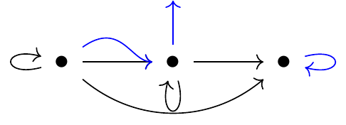
Every object is assigned the unique element of \mathcal{y}(1), i.e. it has one blue arrow emanating from it. And then this arrow is either facing up (it’s returning), or it’s pointing to some morphism leaving that object.

If the monad was \mathtt{list}=\sum_{N:\mathbb{N}}\mathcal{y}^N instead, then every object would be assigned a number N:\mathbb{N}, and we’d see that number of blue hairs—some facing upward, some pointing to outgoing maps. Here’s an example:

As you can see, the first object has two blue hairs, one pointing up (returning) and one pointing to the long outgoing arrow; the second object has no hairs; and the third object has one hair pointing to the identity outgoing arrow.

Now we have a \times-monoid and a \mathbin{\triangleleft}-monoid structure on these hair diagrams: (e,*) and (\eta,\mu) respectively. The e hair diagram has a single hair on each object and each is pointing to the identity map. The \eta hair diagram has a single hair on each object and it is returning (pointing upward).

The *-structure is a map t^c\times t^c\to t^c; it takes two hair diagrams T,T' and produces another. Here’s how. To each object C:c(1) the set of hairs is given by starting with the hairs of T(C), each of which either points upward or along an outgoing map. If it points upward, keep it; if it points along an outgoing map from C, follow it to its codomain, find the hairs of T' there, and add them to the upward hairs you kept from before: each new upward hair is taken as pointing upward from C, and each new arrow in c is composed with the one that got you there using the comonoid structure. Now that you’ve added these together, you’ll find that again each hair either points upward or along a map out of C.

The \mu-structure is a map t^c\mathbin{\triangleleft}t^c\to t^c; given a hair diagram T and, for every object C and every upward-pointing hair x:t[T(C)], another hair diagram T'_x, it produces a hair diagram. Here’s how. To each object C:c(1) we have a set of hairs t[T(C)], and each x:t[T(C)] either points upward or along an outgoing map from C. If it points along a map, keep it; if it points upward, we have another hair diagram T'_x, and we can look at the set t[T'_x(C)] of hairs in it at C; add these to the set of hairs you kept from before, using the monad structure to combine it all. Now that you’ve added these together, you’ll find that again each hair either points upward or along a map out of C.

Can you see why we think of t^c as being about tactics for navigating a category? Let’s say you’re at a terminal working with a bunch of friends down in a category; maybe they’re all together at some object, or maybe some are sitting at one object and some at others. Either way, you have a one-step plan—a tactic—for them to move through the category or to return. Your tactic asks what object they’re sitting at, and then it tells them either to move along the category or to return a specific request to you at the terminal. Given two independent tactics, you can run them in series and collect up the requests; that’s t^c\times t^c\to t^c. And given two dependent tactics (where you have a tactic T:t^c(1) and then another tactic for every request), you can bind them monadically; that’s t^c\mathbin{\triangleleft}t^c\to t^c.

When explaining this to Harrison Grodin, one of this year’s Summer Research Associates at Topos, he suggested that tactics in a proof assistant could be seen in this way. The objects of the category c would be pairs (H\;|\!|\;G), where H is a hypothesis and G is a goal (and the \;|\!|\; doesn’t mean anything more than a comma does; it’s just symbolizing the separation between the hypotheses we have and the goals we want to get to). The morphisms would be legal transformations (H_1\;|\!|\;G_1)\leadsto(H_2\;|\!|\;G_2). For example (A\wedge B \;|\!|\; C)\leadsto(A \;|\!|\; B\Rightarrow C) He wanted to simplify things by taking t\coloneqq\mathcal{y} to be the identity monad. Then a tactic would be to send any current hypothesis-goal state to either a return (“I don’t know what to do here, so I’m returning with the following message: foo”) or to a legal transformation, i.e. to a new hypothesis-goal state. You can run multiple of these in series using *, or you can have ones that depend on the returns of others (i.e. the “foo” return causes some other tactic to run) using \mu.

If all/any of this sounds hand-wavy, you can always just return to the math, found at the beginning of this section.

6 Conclusion

We’ve discussed how raising a polynomial monad to a polynomial power is a lax monoidal operation in two different ways: t^p\times t^q\to t^{p\mathbin{\triangleleft}q} and t^p\mathbin{\triangleleft}t^q\to t^{p\times q}. One upshot is that for any p:\mathbf{Poly}, there is a monad structure on t^p, which I think is pretty interesting. Another upshot is that for a small category (polynomial comonad) c, we find that t^c is not only a monad but also a \times-monoid, also known as an “alternative” in the functional programming community. In the post above, I showed how to think of t^c as telling you about tactics for navigating the category c.

One interesting thing I didn’t discuss is about bicomodules. A (c,d)-bicomodule is a polynomial p equipped with maps c\mathbin{\triangleleft}p\leftarrow p\to p\mathbin{\triangleleft}d satisfying some conditions; such a thing turns out to be a “data migration functor”, which sends d-database instances to c-database instances. But hitting this setup with t^-, we get a \times-bimodule t^c\times t^p\to t^p\leftarrow t^p\times t^d. Just like \mathbin{\triangleleft}-bicomodules form the horizontal maps of an equipment, so too do \times-bimodules form the horizontal maps of an equipment. ⁶ But somehow I find this a bit mysterious. I don’t know what questions I have about these \times-bimodules, except maybe: are there other interesting (t^c,t^d)-bimodules? What do they mean? If anyone reading has thoughts, please say something in the comments below.

This t^c thing—in particular the fact that it is equipped with a compatible monad and monoid structure—is just another example of \mathbf{Poly} producing a very interesting situation that I personally have never encountered before in category theory.

Footnotes

1. The symmetric correlates are \begin{align} \tag{1'} (p_1\mathbin{\triangleleft}p_2)\times q\to (p_1\otimes q)\mathbin{\triangleleft}p_2\\\tag{2'} (p_1\mathbin{\triangleleft}p_2)\times q\to p_1\mathbin{\triangleleft}(p_2\times q)\\\tag{3'} (p_1\mathbin{\triangleleft}p_2)\times q\to (p_1\times q)\mathbin{\triangleleft}(p_2+\mathcal{y}).\end{align}

2. We use (3’) and (evaluation) to get (t^p\mathbin{\triangleleft}t^q)\times p\times q\to((t^p\times p)\mathbin{\triangleleft}(t^q+\mathcal{y}))\times q\to (t\mathbin{\triangleleft}(t^q+\mathcal{y}))\times q Continuing from there, we use (2’), (evaluation), and projection to get (t\mathbin{\triangleleft}(t^q+\mathcal{y}))\times q\to t\mathbin{\triangleleft}((t^q+\mathcal{y})\times q)\cong t\mathbin{\triangleleft}((t^q\times q)+\mathcal{y}\times q)\to t\mathbin{\triangleleft}(t+\mathcal{y}) Finally, we use the unit \eta\colon\mathcal{y}\to t to obtain t+\mathcal{y}\to t, and so we conclude with the multiplication \mu\colon t\mathbin{\triangleleft}t\to t: t\mathbin{\triangleleft}(t+\mathcal{y})\to t\mathbin{\triangleleft}t\to t.

3. Also, colax monoidal functors send comonoids to comonoids, and so strong monoidal functors do both!

4. Polynomial comonads are small categories! See Ahman-Uustalu for the original proof, or this video for details.

5. Thanks to Harrison Grodin for suggesting using strength for the second diagram; this replaced a diagram I had been using, which was more symmetric with the first, but less clear.

6. Since p\times- preserves all colimits, we can take the equipment of monoids and modules in the monoidal category (\mathbf{Poly},1,\times), thought of as a one-object double category.