Solving problem-solving
Our physical world is incredibly complex. Surviving life is a lot about problem-solving, be it waking up in morning and finding your way to the bathroom or solving a math problem for research. We constantly abstract information back and forth from the physical plane to our mental plane for solving these problems. Today I am interested in showing you a way to formalize problem-solving — more specifically, telling the translation story using category theory — and seeing if such abstraction will help enhance the process.
Our physical world is incredibly complex. Surviving life is a lot about problem-solving, be it waking up in morning and finding your way to the bathroom or solving a math problem for research. We constantly abstract information back and forth from the physical plane to our mental plane for solving these problems.
Let us take an example: path-finding. Everyday I (Priyaa) bike to Topos from my home. However, Berkeley was new to me in the beginning! To find my way, I did not think in terms of physical roads, but I opened Google maps, which showed an abstraction of Berkeley. I selected one of the suggested routes, and translated it back into the physical world. So, how can we formalize the process of solving this path-finding problem?
First of all, abstraction leads to construction and use of analogies. I would like to think of Google maps as an analogy of the physical world that is faithful enough to rely on. Path-finding involves translating the problem from the physical world to an analogical map world. The process of constructing analogies is very important in problem-solving, however it is incredibly complex. Therefore, we shall focus on the process of the translating back and forth between the physical and analogical worlds for this scenario.
So, the problem-solving (in simplified terms) involves two steps:
- Abstracting a problem in a forward direction — from the physical world to a map
- Interpreting the solutions in a backward direction — from a map to the physical world
In order to describe this process in a formal sense, we need two pieces:
- a mathematical object to encode problems and the corresponding solutions, and
- a mathematical procedure that specifies how translation between two such domains works:
- translating problems in the forward direction (abstraction) and
- translating its solutions in the backward direction (interpretation).
Let us look at the first piece! My initial search to find a bike route to Topos revealed three routes. So I consider my path-finding to Topos as a problem with three solutions. I can write this in mathematical terms using a monomial: {\sf bike\_to\_work} = \mathcal{y}^{\{ {\sf route1}, {\sf route2}, {\sf route3} \}} or in short form \mathcal{y}^3 where 3 represents an (extensional) solution set with three elements in it. (We shall come back to the symbol \mathcal{y} in a little while.)
However, until I looked at the map, I would not have known that the three routes existed. So, what would the problem monomial {\sf bike\_to\_work} look like before I looked at the map? It would look like this: {\sf bike\_to\_work'} = \mathcal{y}^{\{ \text{bike routes from home to Topos} \}} In this case, the monomial does not list specific routes and is said to have an intensional solution set.1
Now, I may also want to bike to an ice-cream shop, or go buy groceries. These are different path-finding problems each with their own solutions sets. Let’s group all the path-finding problems and formalize them as a single polynomial (polynomial = multiple monomials): \begin{aligned} {\sf bike\_away} &= \mathcal{y}^{\{ {\sf route1}, {\sf route2}, {\sf route3} \}} \\&+ \mathcal{y}^{\{ \text{bike routes home to ice-cream shop} \}} \\&+ \mathcal{y}^{\{ \text{bike routes from home to grocery shop} \}} \end{aligned}
This is how polynomials (also called polynomial functors) are used to encode problems and the solution sets of each problem.
The following figure is a diagrammatic presentation of our polynomial functor {\sf bike\_away}:
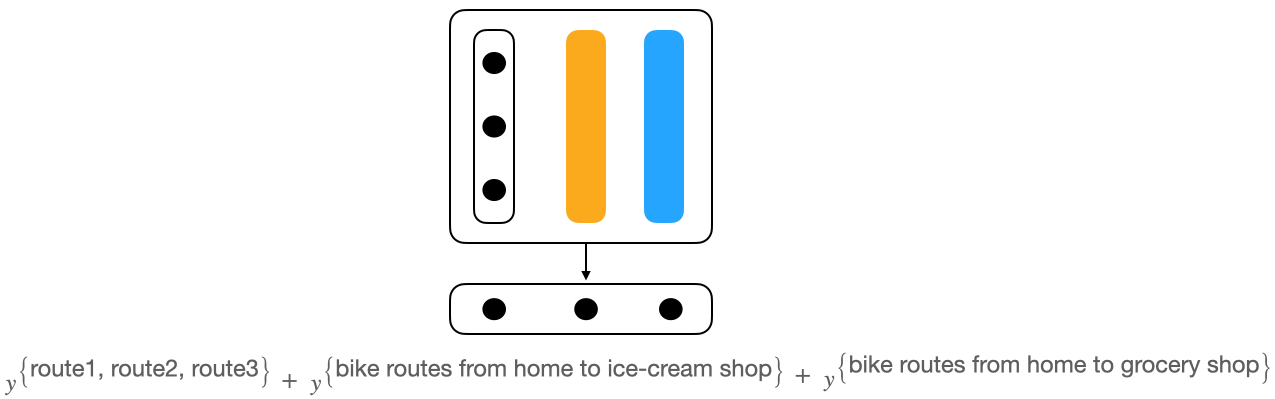
The lower box is the set of path-finding problems. The first dot in the lower box represents path-finding from home to Topos, the second dot represents path-finding from home to ice-cream shop, and the third dot represents path-finding from home to grocery shop. The larger upper box contains the solution sets — each solution set contains desired routes for the path-finding problem directly beneath it. The problem of path-finding to Topos has three solutions — {\sf route1}, {\sf route2}, {\sf route3} — hence, there are three dots in the corresponding solution set. The solution sets where routes are qualified rather than enumerated has a solid color. Note that a solution set can turn out to be empty. If the solution set turns out to be empty, then we write \mathcal{y}^0.
Generally, polynomials can be written as follows: {\sf arena} = \sum_{p:{\sf problem\_set}} \mathcal{y}^{{\sf solution\_set} \text{of $p$}} The term “arena”, or “problem arena”, 2 refers to the mathematical object that contains problems and their solution sets. Think of it as the physical or analogical worlds where events are taking place.
Yayyy! We now know how to encode problems and their corresponding solution sets as a single mathematical object using polynomials. This was the first piece we said we needed.
For the second piece, let us move on to how we formalize the process of problem-solving. Namely, we translate problems from our domain to a second one (from the physical to an analogical world) and then interpret the analogical solutions backwards as actual solutions (from analogical world back into the physical world).
Consider two arenas as follows: \begin{aligned} {\sf problem\_arena} &\coloneqq \sum_{p1: {\sf problem\_set\_1}} \mathcal{y}^{{\sf solution\_set}[p1]} \\{\sf solution\_arena} &\coloneqq \sum_{p2: {\sf problem\_set\_2}} \mathcal{y}^{{\sf solution\_set}[p2]} \end{aligned}
The problem_arena has a problem set called {\sf problem\_set\_1} and for each problem p1 in that set, a solution set called {\sf solution\_set}[p1]. A mathematical specification of problem-solving which we will write as {\sf translate}: {\sf problem\_arena} \to {\sf solution\_arena} is a map of polynomials and consists of two functions:
{\sf t\_forward}: {\sf problem\_set\_1} \to {\sf problem\_set\_2}
This is the abstraction step which maps each problem of {\sf problem\_set\_1} to a problem in {\sf problem\_set\_2}. (for every path-finding problem in the physical world, translate it into a problem in the map world)
For all p \in {\sf problem\_set\_1}, {\sf t\_backward}_p: {\sf solution\_set}[p'] \to {\sf solution\_set}[p],\quad \text{where }p'={\sf t\_forward}(p) This is the interpretation step, where for each problem p in {\sf problem\_set\_1}, the solutions of its translation p' are mapped back into the solution set of the original problem. (For a given path-finding problem, translate the solutions found in the map world to the physical world).
Note that the very type of {\sf t\_backward}_p is determined by the problem p, hence is called a dependent function.
The following is a diagrammatic presentation of a map of polynomials. Follow the arrows that are similarly colored. The {\sf problem\_arena} has problems p, q, and r. The function {\sf t\_forward} maps each of these problems to a problem in the {\sf solution\_arena}. Problem p is mapped to the first problem in the {\sf solution\_arena}. The function {\sf t\_backward}_p maps back the solution set over that first problem to the solution set over p. Problem q is also mapped to the first problem in the solution arena. The function {\sf t\_backward}_q maps back the solution set over that first problem to the solution set over q. Problem r is mapped to the second problem in the {\sf solution\_arena}. The function {\sf t\_backward}_r maps back the solution set over that second problem to the solution set over r. Neat, isn’t it?
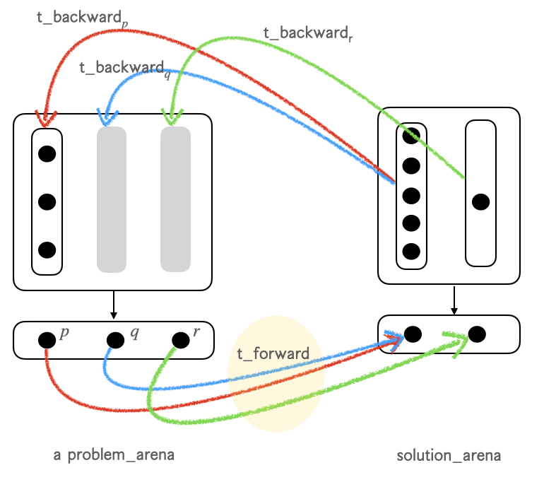
We now know how to translate problems in a forward direction and solution in a backward direction, using polynomial maps. This was our second piece. Yayy!
Did you notice — we started with the idea that abstraction is something we do in everyday life to solve problems but we ended up abstracting problem-solving process itself?!
In the next post, we shall build on polynomials to describe more complex forms of translations for problem-solving. For example, suppose I want to pick a coffee en-route to Topos. What is the polynomial description of this problem-solving process where the solutions (routes) must be composed — home to coffee shop followed by coffee shop to Topos? Polynomials provide elegant ways of describing such complex translations which will be theme of the next post!
P.S. An ode to polynomials
A functor p: {\sf Set} \to {\sf Set} is a polynomial if there exists an arbitrary set I and a family of sets (A_i)_{i:I}, p \simeq \sum_{i:I} \mathcal{y}^{A_i} where \mathcal{y}^{A_i} := {\sf Set}(A_i, -).
Polynomial maps are natural transformations between these functors.
Acknowledgement: Thank you, Beth Williams, for editing this draft and for your perspective! And I attribute the map analogy to the view of downtown Berkeley, out of my office window!
Footnotes
The difference between extensional and intensional sets is whether the set is specified by enumerating all its members or by specifying it in terms of a syntax and rules. For example \{2,3,5,7\} and \{n:\mathbb{N}\mid n<10\text{ and }n\text{ is prime}\} are extensional and intensional versions of the same set. One could define a bike route intensionally as a route (some syntax of streets and turns) subject to the rule of being bike-friendly (some rules about traffic, etc.)↩︎
“Arena” is the name that David Jaz Myers uses for similar objects in his Categorical Systems Theory book.↩︎