Building dynamic structures
In our day-to-day lives, we all interact with many systems where the structure of the system changes based on external or internal factors. How do we make sense of structures that can change in this way? In mathematics, we often assume the structure we’re working with is “fixed” to some extent, and here we want the exact opposite: structures that can change. This summer, as part of Topos’ 2023 Summer Science Research Associates cohort, I spent a lot of time with David thinking about and working on this problem, and I’m excited to discuss a streamlined mathematical approach to describing and building structures that can be updated in this way.
In our day-to-day lives, we all interact with many systems where the structure of the system changes based on external or internal factors. Each of our bodies is an immense network of cells, human and bacterial, in constant dialogue with internal and external factors, sometimes dying, mutating, or being created. On a grander scale, an ecological system involves many actors — the flora and fauna, the climate, the geology, ect. — and the interlinking web of relations changes, slowly, over time, as new species evolve, the climate drifts, and extant species compete for survival. In a prediction market, the reputations of involved guess-makers change and update over time based on the success or failure of their guesses. When optimizing an artificial neural network using gradient descent, the weights and biases involved are constantly being updated based on the training data.
How do we make sense of structures that can change in this way? In mathematics, we often assume the structure we’re working with is “fixed” to some extent, and here we want the exact opposite — structures that can change. This summer, as part of Topos’ 2023 Summer Science Research Associates cohort, I spent a lot of time with David thinking about and working on this problem, and I’m excited to discuss a streamlined mathematical approach to describing and building structures that can be updated in this way.
1 Dynamic arrangements
To understand how we can change organizational structure, then, let’s describe the structures we want to be able to change in an example. Let’s imagine we have sets A, B, and C, and two interfaces p_1 = Ay^B \qquad p_2=B^2y^C where B^2 = B \times B. The polynomial p_1 inputs things of type B and outputs things of type A, and p_2 inputs things of type C and outputs a pair of things of type B. We can arrange these two interfaces into a system in multiple different ways. For example, our new interface, System, could input something of type C and output things of type A, B, and thus be a polynomial \text{System} =ABy^C
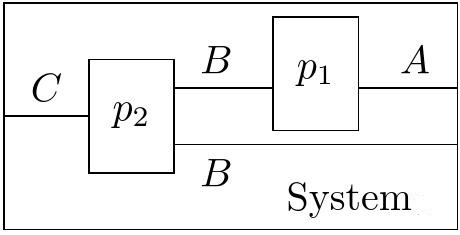
The wiring diagram above tells us exactly how we’ll put together p_1 and p_2 to get this arrangement. That is to say, arrangements as in Figure 1 are polynomial morphisms p_1 \otimes p_2 \to \text{System} A polynomial morphism AB^2y^{BC} \to ABy^C consists of two set maps. The first of these is a map AB^2 \to AB that tells you what the outputs of the entire system are, given the outputs of the components. Here, we can see that if p_1 and p_2 are outputting (a,b,b'), the output of the system will be (a,b). The second map is a function AB^2C \to BC, that says how, if the components are outputting a thing of type A and two things of type B, and the system is being input some thing of type C, what inputs we should feed into the components. Here, this is (a,b,b',c) \mapsto (b,c). However, this arrangement is static, in the sense that it is a fixed polynomial morphism, and the component maps do not change — we cannot “re-wire” this diagram. But we could imagine gluing together our two interfaces in more than one way. For instance:
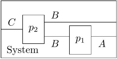
Here, as opposed to p_1 inputting the first output of p_2, it inputs the second output. Given a set S with two objects x, y we could then define a mapping \{x,y\} \to \{\text{Arrangement}_0, \text{Arrangement}_1\} that sends x to the first arrangement, \text{Arrangement}_0, and y to the second arrangement, \text{Arrangement}_1. In fact, this is already halfway to the description of a dynamic arrangement. A dynamic arrangement is an arrangement that can be changed by internal and external factors. To be more precise, a dynamic arrangement will have a set S of states, so that each state s:S corresponds to an arrangement, as above. However, we also have some way of updating the state based on what has occured in the arrangement — what has flowed out of and within the arrangement. This “update” will be a set function with codomain S. Dynamic structures as defined in (Shapiro and Spivak 2022) are thus structures where we can associate dynamic arrangements to objects.
In fact, the training of an artificial neural network and the running of a prediction market each are a form of a dynamic structure — a dynamic monoidal category and a dynamic operad, respectively (Shapiro and Spivak 2022). For artificial neural networks, the state is the set of weights and biases, which is updated using backpropagation based on the performance of the model as it is trained. For prediction markets, the states are the current reputations of the involved participants, which update and change based on the performance of their predictions. What other structures have dynamic arrangements, and what are the building blocks necessary to find such a structure?
2 Building dynamic structures
So, from (Shapiro and Spivak 2022), we have two specific examples of dynamic structures in artificial neural networks and prediction markets. We also philosophically have many additional examples of things that feel “dynamic”-ish: the many structures that adapt and change based on how they are used, such as the cells in the body, the environment, and so on. We would like to find many more such dynamic structures. As it turns out, it’s enough to have the structure of a reverse derivative category.
The categorification of the reverse derivative, an important construction in machine learning that is used for backpropagation, was first presented in (Cockett et al. 2020). To start out with, a reverse derivative category \mathcal{A} has the underlying structure of a Cartesian left-additive category. So \mathcal{A} is a monoidal category where the monoidal product is given by the categorical product such that each object a of \mathcal{A} is equipped with a commutative monoid structure, with addition +_a: a \times a \to a and zero 0_a: 1 \to a. We’ll further equip \mathcal{A} with a reverse differential combinator, a device that turns any morphism f: A \to B into a morphism R[f]: A \times B \to A. The reverse differential combinator must satisfy a healthy list of axioms that make it behave, appropriately enough, like a reverse derivative from machine learning: that the reverse derivative of a sum is the sum of the reverse derivatives, that the reverse derivative is linear in its secon argument, the reverse analogue of the chain rule, and so on.
For an example of a reverse derivative category, let R be some commutative rig1. You can then consider the category \mathbf{POLY}_R of polynomials with coefficients in R. The objects of \mathbf{POLY}_R are natural numbers n. Given any two natural numbers n and m, a morphism P: n \to m in \mathbf{POLY}_R is an m-tuple of polynomials in n variables with coefficients from R: P = \langle p_1(\overline{x}), ..., p_m(\overline{x}) \rangle where p_i \in R[x_1, ..., x_n] for 1 \leq i \leq m. We should pause here to be very clear that \mathbf{POLY}_R is the category of polynomials with coefficients in R, where “polynomial” here has the ordinary, abstract-algebra sense, so we should be careful to mentally distinguish between the polynomials that are morphisms in \mathbf{POLY}_R and our polynomial functors. \mathbf{POLY}_R is then a Cartesian left-additive category, where composition is given by polynomial composition and the monoidal product given by regular addition of natural numbers . Moreover, \mathbf{POLY}_R is a reverse derivative category (Cockett et al. 2020), where the reverse derivative of P: n \to m is R[P]: m \times n \to n, an n-tuple of polynomials in m+n variables with coefficients in R, defined using the partial derivatives of polynomials: R[P] : \left \langle \sum_{i=1}^m \frac{\partial p_i}{\partial x_1} (\overline{x}) y_i, ..., \sum_{i=1}^m \frac{\partial p_i}{\partial x_n} (\overline{x}) y_i\right \rangle
For instance, an arrow P=2 \to 3 in \mathbf{POLY}_{\mathbb N} is a 3-tuple of polynomials in {\mathbb N}[x_1, x_2], such as P = \langle 2x_1^2x_2^2 + 3x_1, 8x_1^2x_2+4x_1x_2, x_1+2x_2 \rangle The reverse derivative R[P] of P is an arrow 5 \to 2 in \mathbf{POLY}_{\mathbb N}, so a tuple of polynomials in five variables x_1, x_2, y_1, y_2, y_3: R[P] = \langle (4x_1x_2^2+3)y_1+(16x_1x_2+4x_2)y_2 + y_3, 4x_1^2x_2y_1+(8x_1^2+4x_1)y_2 + 2y_3 \rangle
Since our goal is to build a dynamic structure with the same objects as our original reverse derivative category, and since dynamic arrangements have polynomials as a fundamental component, we want some way to associate a polynomial to every object A of \mathcal{A}. As an intermediate, we first want a product-preserving functor F from \mathcal{A} to \mathbf{Set}. Luckily for us, there’s at least as many product-preserving functors F as there are objects of \mathcal{A}, as the representable copresheaves are product-preserving. Equipped with a product-preserving functor F, we can assign to each object A of \mathcal{A} the polynomial F(A)y^{F(A)} — this is a machine that inputs and outputs elements of the set F(A).
For two objects A and B of our reverse derivative category \mathcal{A}, we developed a dynamic arrangement as follows. Our states are quadruples (M, \text{move}, f, m), where M is an object of \mathcal{A}, \text{move} is a set function F(M) \times F(M) \to F(M), f is an arrow f: M \times A \to B in \mathcal{A}, and m is one element of F(M). We can view F(M) as a set of parameters, so m: F(M) is a specific choice of parameter. The arrangement corresponding to this state is then a polynomial morphism F(A)y^{F(A)} \to F(B)y^{F(B)} given by F(A) \xrightarrow{m\times\text{id}} F(M)\times F(A) \xrightarrow{F(f)} F(B) and F(A)\times F(B) \xrightarrow{m\times\text{id}} F(M)\times F(A)\times F(B) \xrightarrow{F(R[f])} F(M)\times F(A) \xrightarrow{\pi} F(A)
This says that given an output of the interface F(A)y^{F(A)} we can get an output of F(B)y^{F(B)} by applying F(f)(m,-). Additionally, given an input of F(B)y^{F(B)} and an output of F(A)y^{F(A)}, we can get an input of F(A)y^{F(A)} essentially just using the parameter m and the reverse derivative of f. When we update this state based on what flows in and out of the arrangement, we’ll keep our parameterizing object M and distinct maps move and f unchanged, and just update the choice of parameter m. Our update map \text{upd}: F(A) \times F(B) \to F(M) will produce a new parameter m' to replace m, by composing our \text{move} function — which tells us how to change the parameter based on the inputs and outputs of the arrangement — with the reverse derivative: F(A)\times F(B) \xrightarrow{m;F(R[f])} F(M)\times F(A) \xrightarrow{\pi;\Delta_{F(M)}} F(M)\times F(M) \xrightarrow{\text{move}} F(M)
This particular construction actually recovers one of our examples from before, artificial neural networks, where the parameterizing element m:F(M) is the particular weights and biases. The move function, which we use to update our weights and biases, will be “Euler’s method” according to a learning rate. In fact, this summer we were able to show that the construction I’ve described here on reverse derivative categories generalizes quite a bit, and we’re able to build dynamic structures out of more general ingredients. The full construction is outlined in a forthcoming paper. This is exciting, since it helps us see what sort of building blocks we need to build the dynamic structures that are all around us.
References
Footnotes
A rig is a ring without additive inverses, a.k.a. a semiring.↩︎