Composing springs
Physical systems are often composed of many interacting subsystems. In this post, we take a peek at the math and the software implementation for composing systems of springs using decorated cospans.
1 Physics is hard
In my 16+ years of formal education, the lowest grade I’ve ever received was in General Physics I, which covered “vectors, kinematics, Newton’s laws and dynamics, conservation laws, work and energy, oscillatory motion,…”
There’s a textbook diagram that stands out in my memory as example of why this course was so challenging for me. The diagram contains a bunch of pulleys (where “a bunch” means like “3”) all connected to each other. One pulley made sense. Two pulleys, okay. But once there were many pulleys, many masses, and hence many forces to track, I would invariably lose my way. I understood each of the components, but in my physics education there was not a practice of explicitly representing their composition. Instead the composition pattern was implicit to the solving process, and so computing the composition of many pulleys was largely heuristic rather than a formal and legible process. Thankfully applied category theory is here to help me out.
Consider for example the problem of determining the oscillation of a spring on Earth. Here’s how undergraduate-me would have solved that problem:
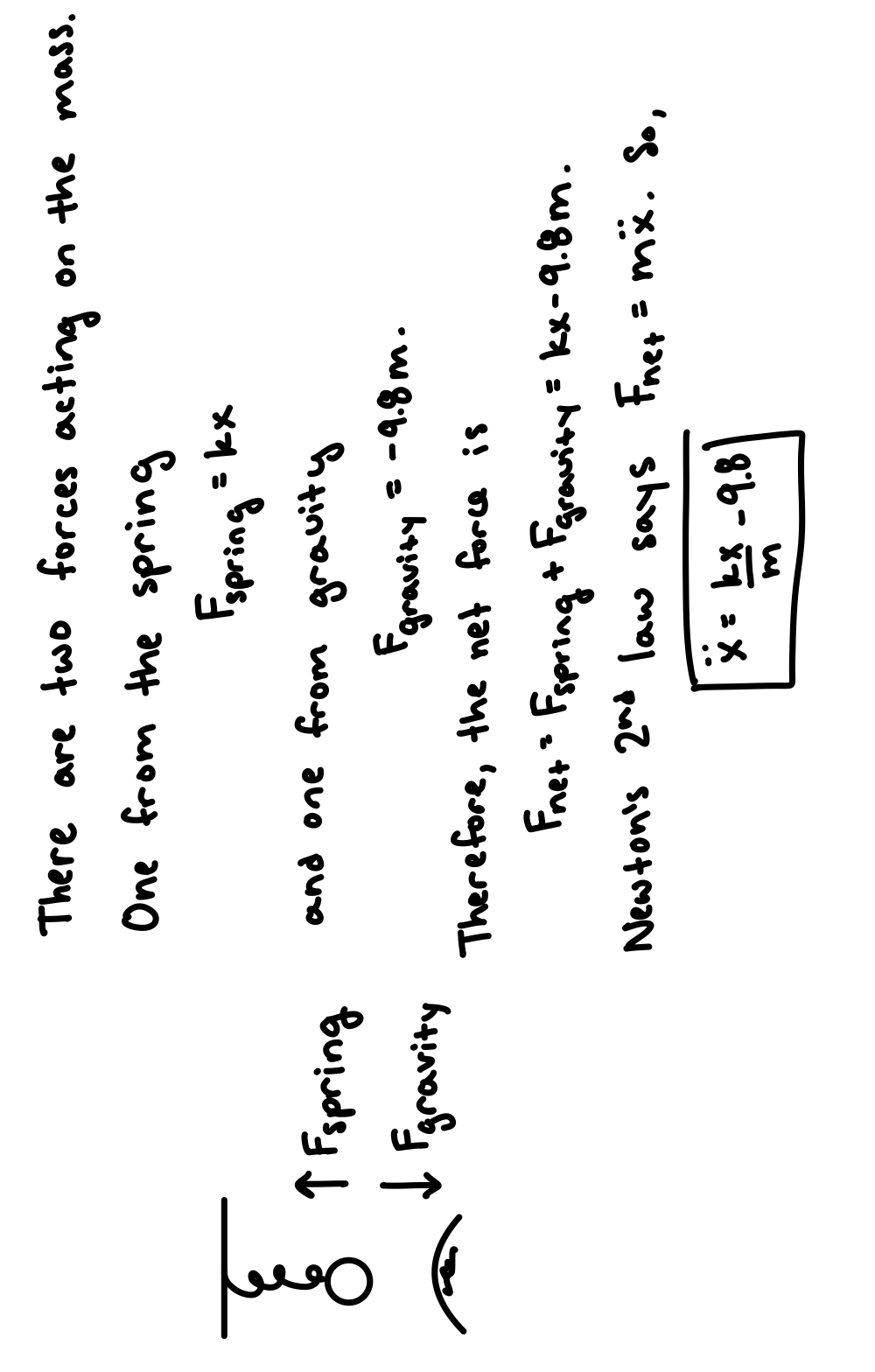
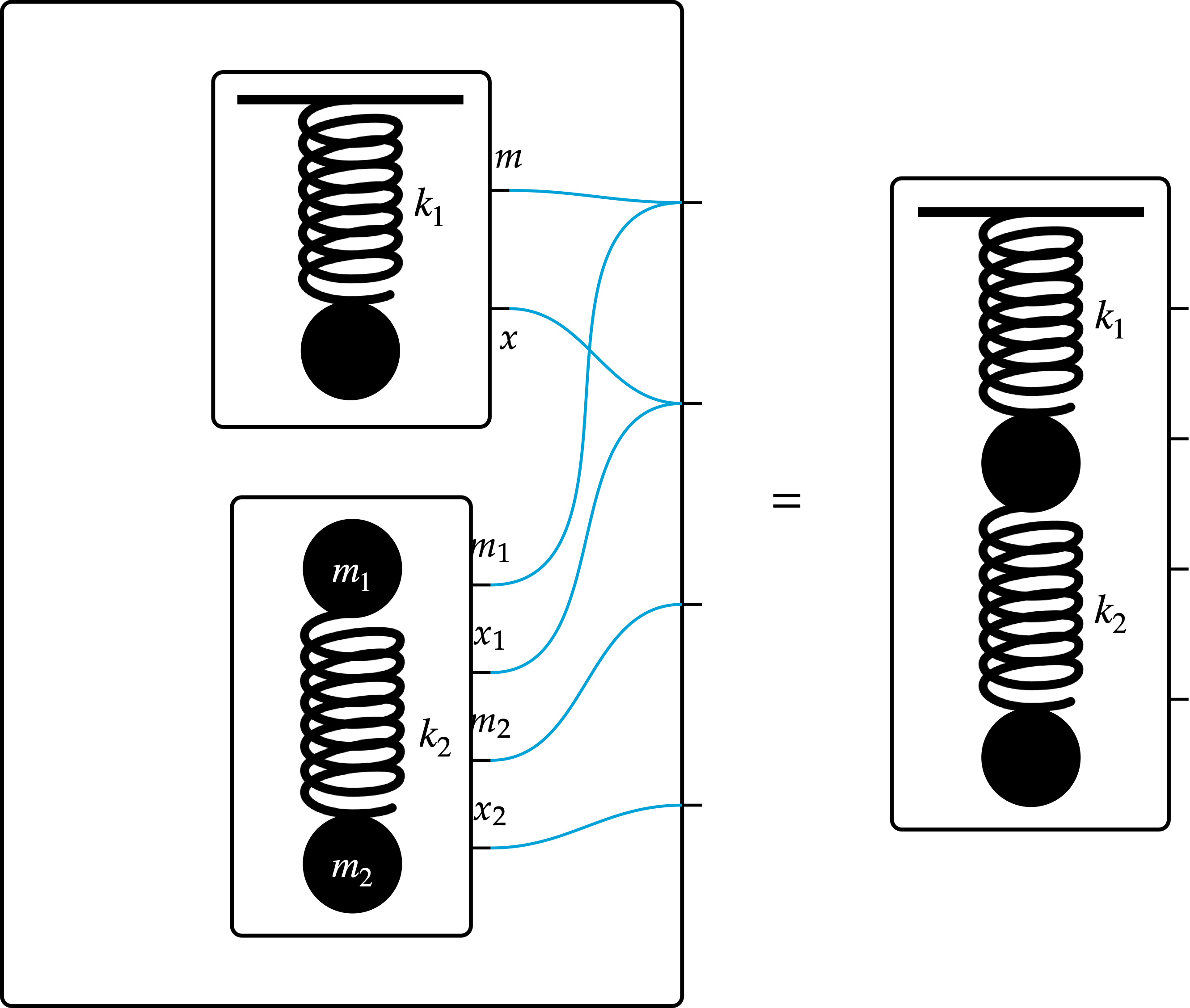
That this system has two components (the spring and the effects of gravity) with a specified interaction (the mass in the two systems are the same) is hidden in the sum F_\text{total} = F_\text{spring} + F_\text{gravity}. Roughly,

We can formalize the interaction using an undirected wiring diagram (UWD) like this:
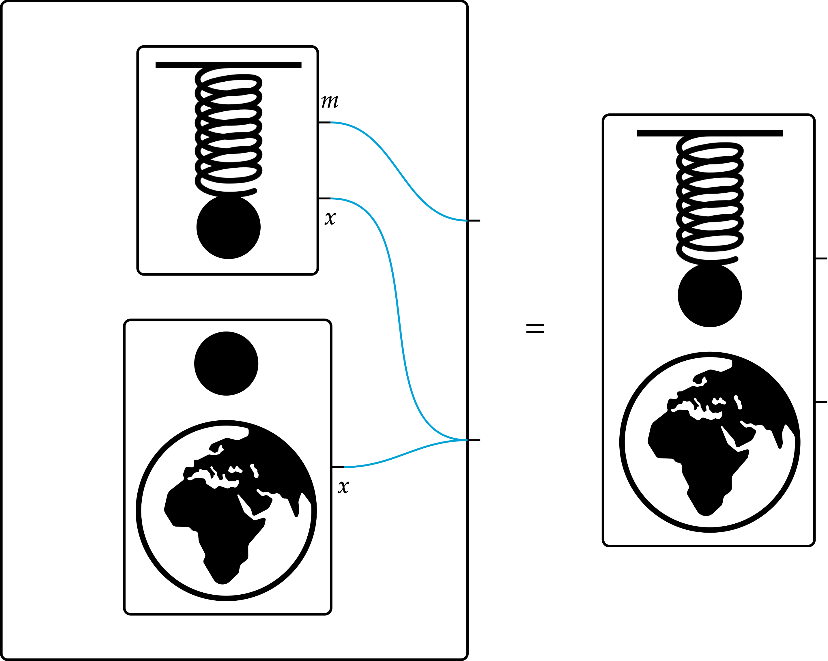
where m represents the mass and x represents the position of the mass. That the ports labeled x in each component system are wired together means that they are identified in the composite system.
We can formalize the component systems as differential equations using the operad algebra of resource sharers:
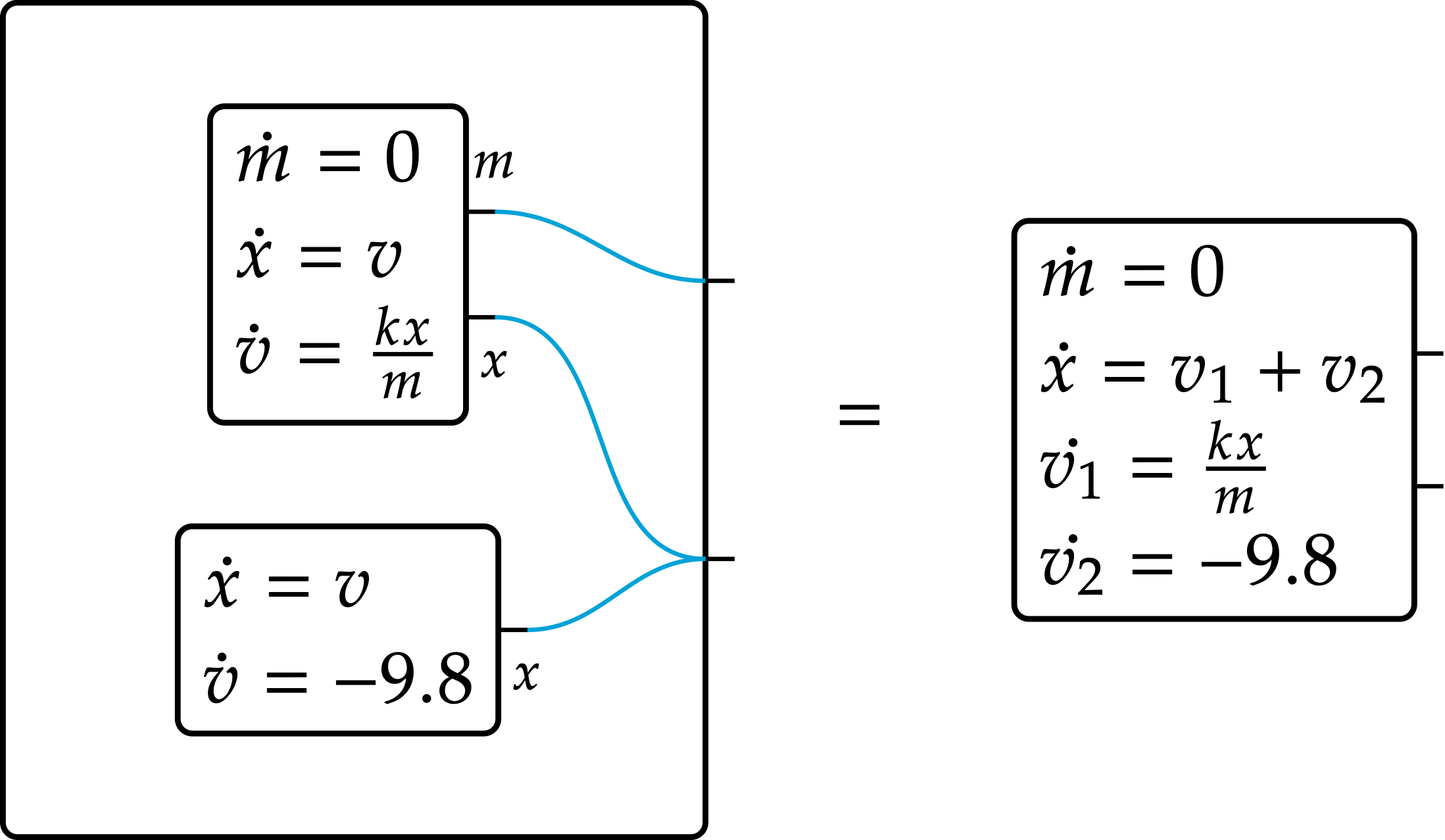
To solve this physics problem, I provide the components and interactions on the left-hand side, and the resource sharing machinery defines the composite system on the right. Then I can solve, \ddot x = \dot v_1 + \dot v_2 = \frac{kx}{m} - 9.8.
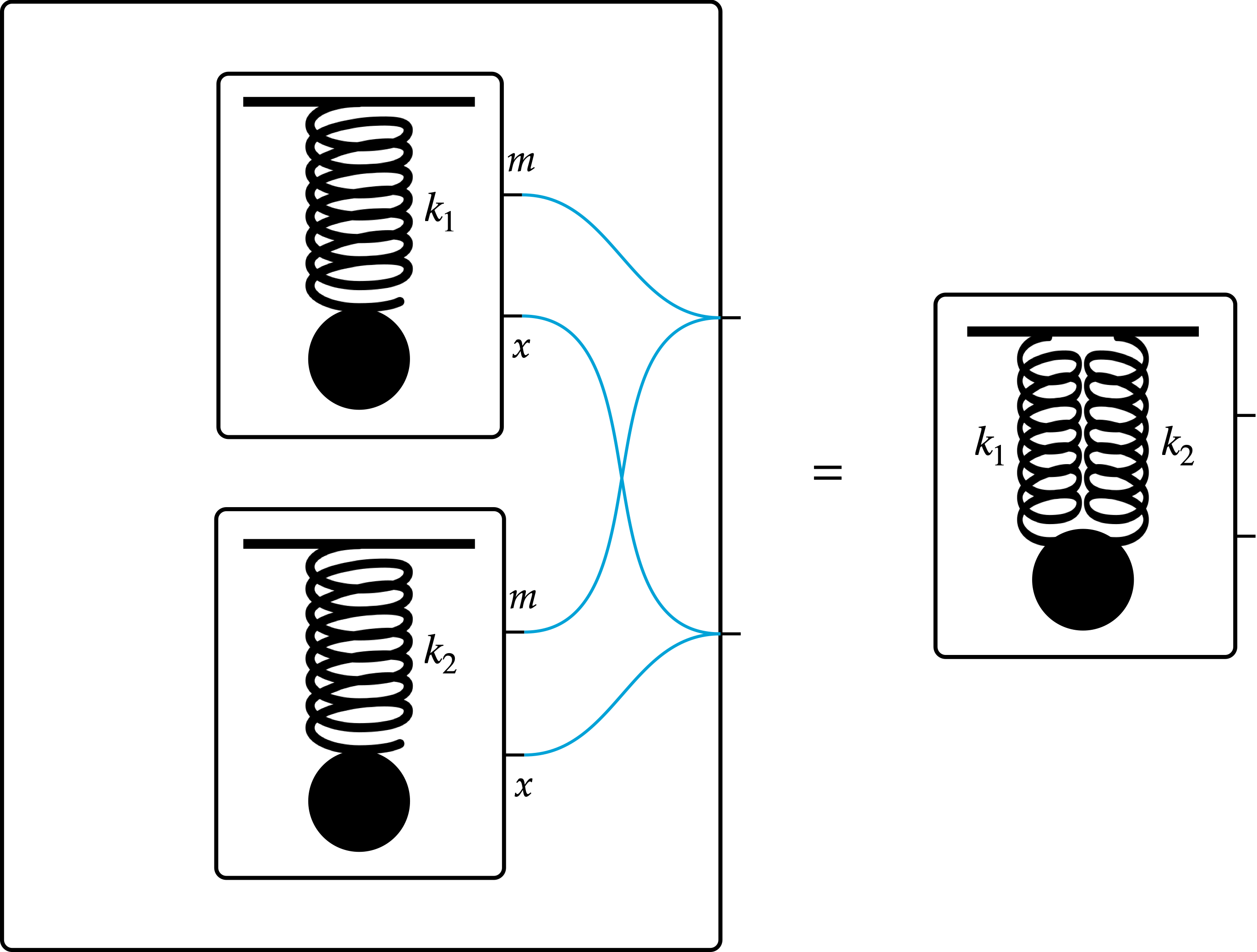
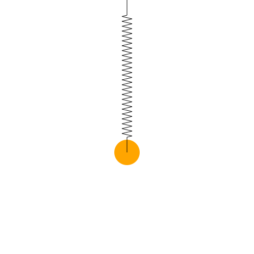
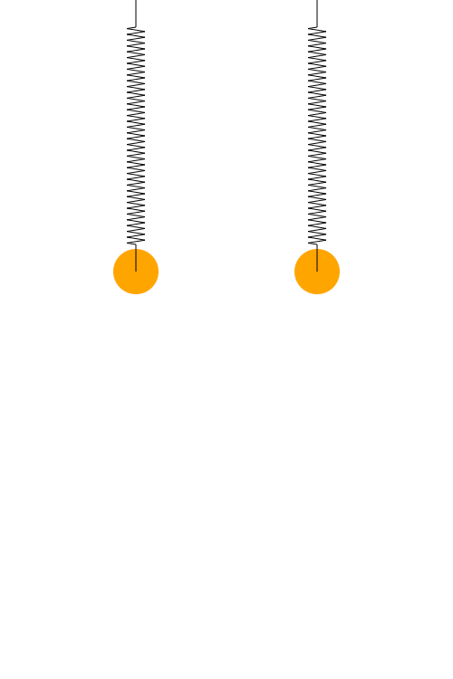
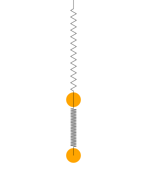
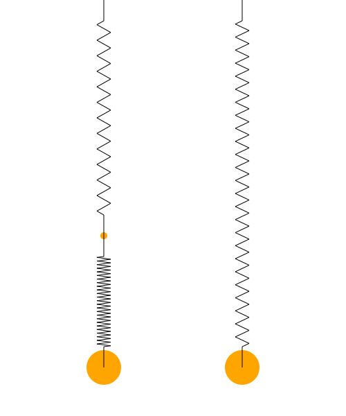
Using the same strategy of explicitly representing the components and their interactions, we can also understand two springs in parallel and in series:
2 Implementation in AlgebraicDynamics
In AlgebraicDynamics we can translate our whiteboard diagrams into compilable code in order to compute and then simulate the composite systems. Let’s do this for the spring on Earth.
First we implement the anchored spring as a ContinuousResourceSharer which specifies the interface and a particular choice of system with that interface.
function anchored_spring_dynamics(k)
  (u,p,t) -> begin
      mass, pos, vel = u
      [0., vel, -k*pos/mass]
  end
end

anchored_spring(k) = ContinuousResourceSharer{Float64}(
    [:mass, :pos],               # interface
    3,                           # number of state variables
    anchored_spring_dynamics(k), # dynamics
    [1,2]                        # port map
)
Let’s break down this specification:
[:mass, :pos]indicates that the interface of this system has two exposed ports labeled:massand:pos.3indicates that there are three state variables.anchored_spring_dynamics(k)returns a Julia function that defines the vector field for an anchored spring with spring constant k.[1,2]defines the port map, which indicates that the first port exposes the first state variable and the second port exposes the second state variable.
Given an initial mass, position, and velocity for the spring, we can use the DifferentialEquations Julia package to solve the system and plot the trajectories of the exposed state variables over time.

As expected the mass remains constant throughout the run while the position oscillates. While this plot is indicative, it is more fun to use Javis to animate our spring.
Now we’re ready for composition. While ContinuousResourceSharers represent single systems, UndirectedWiringDiagrams represent an interaction pattern. Once the primitives systems and the interaction patterns are defined, we can compose using the oapply method.
# Define the gravitational system
gravity_model = ContinuousResourceSharer{Float64}([:pos], 2, (u,p,t) -> [u[2], -9.8], 1:1)

# Define the interaction pattern as a UWD
interaction = @relation (mass, pos) begin
  spring(mass, pos)
  gravity(pos)
end

# Compose
spring_on_earth = oapply(interaction, Dict(:spring => spring, :gravity => gravity))
Catlab automatically generates a visual of the UWD interaction.

The animation of a solution for the composite system spring_on_earth is exactly what we expect: the spring on Earth oscillates with the same frequency as the original spring but with a lower equilibrium point.
2.1 Springs in parallel
As shown in the introduction, we can construct springs in parallel as the composition of two anchored springs whose positions and masses are identified. This interaction pattern is encoded by the following UWD.

Now the implementation of springs in parallel is just a few lines of code.
k1 = 10.0; k2 = 20.0
spring1 = anchored_spring(k1)
spring2 = anchored_spring(k2)

interaction = @relation (mass, pos)  begin
  spring1(mass, pos)
  spring2(mass, pos)
end

parallel_springs = oapply(interaction, Dict(:spring1 => spring1, :spring2 => spring2))
A nice test of this example is to compare our springs in parallel to a single spring with spring constant {k_1 + k_2}. According to physics, these have the same behavior. And indeed that’s what we see.
2.2 Springs in series
For springs in series, we have an anchored spring connected to a free spring1 in which one anchor point of the free spring is the mass of the anchored spring. This interaction pattern is encoded by the following UWD.

Again, the implementation of springs in series is now just a few lines of code:
k1 = 10.0; k2 = 20.0
spring1 = anchored_spring(k1)
spring2 = free_spring(k2)

interaction = @relation (m1, m2, p1, p2) begin
  anchored_spring(m1, p1)
  free_spring(m1, p1, m2, p2)
end

series_springs = oapply(interaction, Dict(:anchored_spring => spring1, :free_spring => spring2))
When both masses are 5 grams, we can simulate the springs in series and animate the results:
If the mediating mass is negligible, then our springs in series have the same behavior to a single spring with spring constant \frac{k_1 k_2}{k_1 + k_2}.
Pretty cool!
3 The operad algebra of resource sharers
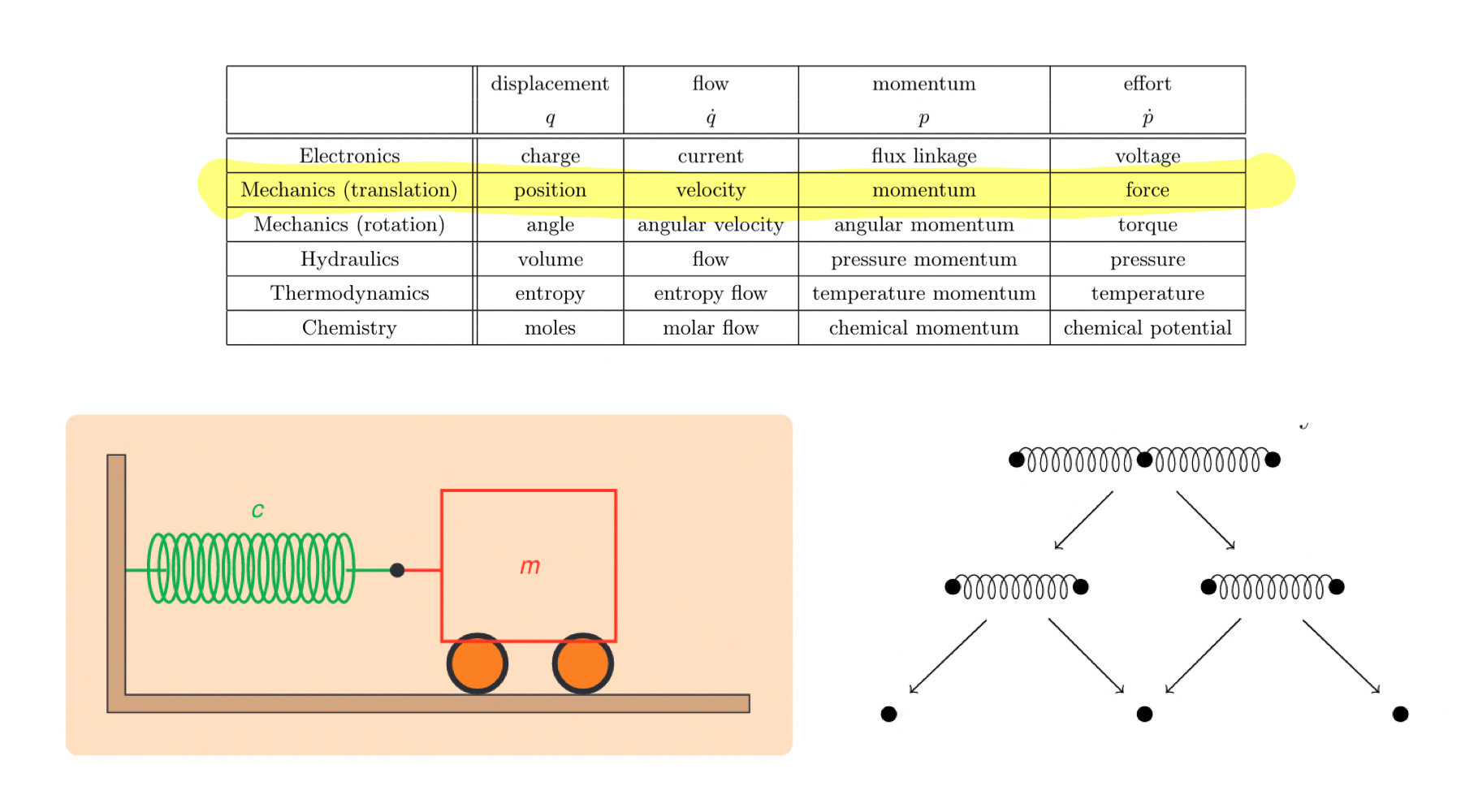
In one of the first papers on decorated cospans — an applied category theory tool for composing systems in science and engineering — Baez and Fong laid out a table of analogies between electrical, physical, thermodynamic, chemical, and hydraulic systems (Baez and Fong 2018). While in the paper, they focus on electrical systems, the analogy suggests a diagrammatic mathematics for composing physical systems as well. This work was seeded by Jan Willem’s pamphlet Tearing, Zooming, Linking (Willems 2007) where he throws out the input/output approach to system composition and instead focuses on what I call resource sharing, which is the type of composition we’ve seen so far in this post.
In the resource sharing paradigm of composition, systems compose by identifying parts of their components. Imagine if we said “your hand and my hand, they’re actually the same hand!” then we would form a composite system by identifying our hands. Our hand is the shared resource.
Composing springs is time-honored example in the study of resource sharers.
In the remainder of this post, we flesh out the mathematics of the algebra of resource sharers, which clarifies what the rules are for (1) drawing interaction patterns and their component systems and (2) computing the composite system. In other words, it specifies what can fill a box, how boxes can be connected, and how the composite system is defined.
The operad algebra of resource sharers is a functor R: \mathcal{O}(\mathsf{Cospan}_{\mathsf{FinSet}}) \to \mathcal O(\mathsf{Set}). At its core, it is the cospan algebra induced by the decorated cospan category2 \mathsf{Open}(\mathsf{Dynam}) introduced in (Baez and Pollard 2017)3.
The action of R on types tells us what can we compose. Types in \mathcal{O}(\mathsf{Cospan}_{\mathsf{FinSet}}) represent system interfaces. In particular, a type in \mathcal{O}(\mathsf{Cospan}_{\mathsf{FinSet}}) is a finite set M, and it represents an interface with M exposed ports. Then the set R(M) is the “set of systems with interface M”, i.e. the “set of systems with M exposed ports.” In this case, a system with M exposed ports consists of:
- A finite set of state variable S \in \mathsf{FinSet}.
- A vector field on the state space v: \mathbb{R}^S \to T\mathbb{R}^S.
- A port map p: M \to S which assigns to each exposed port a state variable that it exposes.
Therefore, R(M) = \{(S \in \mathsf{FinSet}, v: \mathbb{R}^S \to T\mathbb{R}^S, p: M \to S)\}.
The action of R on morphisms tells us how systems interact. Morphisms in \mathcal{O}(\mathsf{Cospan}_{\mathsf{FinSet}}) represent interaction patterns between systems. Recall that a morphism \phi: M_1, ..., M_n \to N in \mathcal{O}(\mathsf{Cospan}_{\mathsf{FinSet}}) is a cospan of finite sets M_1 + ... + M_n \to J \leftarrow N where J represents a set of junctions. Given such an interaction pattern \phi, R(\phi): R(M_1) \times ... \times R(M_n) \to R(N) is a set map which takes a systems of types M_1,..., M_n and returns a system of type N. In other words, R(\phi)(s_1,...,s_n) is the composition of systems s_1,..., s_n according to the interaction pattern \phi. And what does R(\phi) actually do? It identifies variables joined at junctions and adds their dynamics. Checkout (Libkind et al. 2021) for the details.
We can now repeat the example of a spring on Earth, but this time with more mathematical depth.
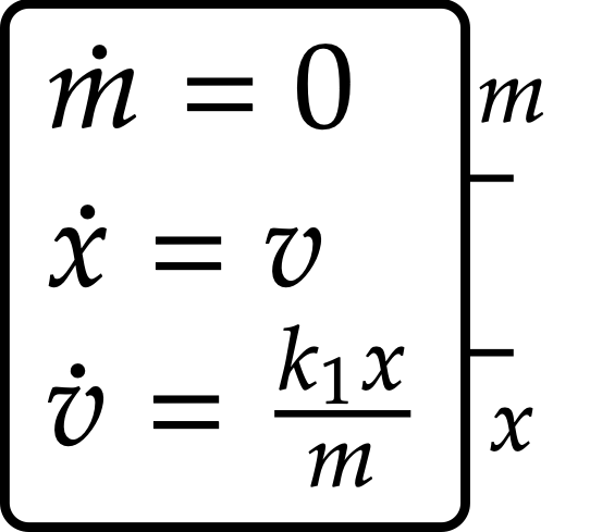
Let’s write an anchored spring with spring constant k as an element of R(2). This system has three state variables S = \{m, x, v\} corresponding to the mass, position (relative to its equilibrium), and velocity of the free endpoint. The vector field is given by \dot m = 0, \qquad \dot x = v, \qquad \dot v = kx/m. This vector field says “the mass doesn’t change, the position changes according the velocity, and the velocity changes according to Hooke’s law.” Finally the system has two exposed ports which expose the mass and position. This means that the mass and the position of the spring’s endpoint are exposed for “sharing” or being identified with exposed quantities of other open systems. However, the velocity is internal to the system and cannot directly affect nor be affected by other systems.
The anchored spring we defined in Example 1 is living in vacuum. There is no gravitational force acting upon the mass. Let’s define a spring on Earth by composing the anchored spring with a system representing gravity.
First, we define the gravitational system. It has two variables \{x, v\} again representing a position and a velocity. Its dynamics are given by \dot x = v and \dot v = -9.8. Finally, this system will have only one exposed port which exposes the position.
How do the anchored spring and the gravitational systems interact? The naming of variables gives us a hint. The positions of the masses in the two systems are the same! To formalize this interaction between systems, we define a UWD in which the ports exposing the two position variables map to the same junction.
Finally, we compose the systems according to the action of R on this interaction pattern. Following the slogan “identify variables and add their dynamics,” we determine the variables of the composite system by identifying the variables of the primitive systems which are joined at junctions. This process gives us four variables: \{m, x, v_1, v_2\}. m represents the mass defined in the anchored spring. The positions of the anchored spring and of the gravitational systems have been identified and are now both represented by a single variable x. However, the velocities of the two systems were not identified. This gives us two velocities in our composite system. The velocity of anchored spring is represented by the variable v_1, and the velocity of the gravitational system is represented by the variable v_2. As is clear from the picture, m and x are the exposed variables of the composite system.
So what are the dynamics of the composite system? The dynamics of m, v_1, and v_2 are directly copied from the primitive systems: \dot m = 0, \qquad \dot v_1 = kx/m,\qquad \dot v_2 = -g. But how should the positions change over time? Recall that x represents both the position of the anchored spring and the position of the gravitational system. Our slogan says “add their dynamics”. So let’s do that! \dot x = v_1 + v_2.
4 Resources
If you want to learn more about AlgebraicDynamics and the operad algebras it implements checkout the following resources:
- (watch) Happy Birthday AlgebraicDynamics.jl is a talk I gave at Topos’s Berkeley Seminar celebrating AlgebraicDynamics’s first birthday.
- (read) Operadic Modeling of Dynamical Systems: Mathematics and Computation gives a full account of several operad algebras for composing dynamical systems as well as their implementations in AlgebraicDynamics.
- (diy) Checkout AlgebraicDynamics on GitHub. In particular, this notebook reproduces the examples shared in this blog post.
References
Footnotes
The free spring has a mass, position, and velocity for both ends of the springs, so it has 6 state variables and 4 exposed ports.↩︎
Every decorated cospan category is a hypergraph category and every hypergraph category is 1-equivalent to a cospan algebra (Fong and Spivak 2019).↩︎
You can find more details about other of the algebras implemented in AlgebraicDynamics.jl in (Libkind et al. 2021).↩︎