Jump monads: from conjugation to dependent types

Abstract

The world of polynomial functors often seems so rich that it should contain the whole universe, and there are some tantalizing suggestions that, in fact, it does. Given a dependent type theory, we can follow Steve Awodey and encode its syntax into a “universe polynomial” indexed by the types of the theory, and whose summands represent the terms of each type. How far can we follow this idea? How does dependent type theory relate to the categorical structure of polynomials?

Edit, 2022-02-03: The main example in this post—that there is a self-distributive law on the free monoid monad—is not correct. A couple weeks ago while writing an extension of these ideas up into a paper, I realized that this claim would imply that the “type theoretic axiom of choice” is somehow an equality where it isn’t: it’s just an isomorphism. And this week, when telling Brandon Shapiro about the issue, he pointed me to an article by Maaike Zwart and Dan Marsden verifying that it indeed cannot be fixed. So take everything below with plenty of salt.

At the 2021 Workshop on Polynomial Functors, Steve Awodey gave a talk called Polynomial functors and natural models of type theory. For the past year or so, I’ve been using polynomial functors to think about dynamics, decisions, and data; it put quite a bee in my bonnet to think that I could add dependent types to the list.

I’ve been hoping to find a way to make the dynamical systems “speak” to each other in a native or internal language, rather than simply by sending arbitrary tokens. Steve’s talk seemed quite relevant, because rather than discussing the semantics of dependent types, he was showing that the syntax — the language itself — could be constructed as a polynomial that I’ll call u (for “universe”) that has certain properties. For example, by giving u the structure of a monad, we somehow get a unit type and sum types in our language.

In this post I’ll try to explain the above ideas (another place to look is Clive Newstead’s thesis). I’ll also say what I came up with when trying to understand Steve’s idea from my own perspective. In fact, what really made a difference for me was André Joyal’s question during Steve’s talk. He asked “What happened to the distributivity law that we love between sum and product in this setting?” We’ll see that, while I haven’t pinned down exactly what Steve has done, much of the structure comes from a distributivity structure u\triangleleft u\xrightarrow{\nabla} u\triangleleft u of the universe polynomial with itself. Indeed, the \Pi type-former arises from this distributivity structure and then naturally distributes over \Sigma.

When this self-distributive monad satisfies a certain additional property, I started calling it a jump monad, because it kind of looks like this: (A,B)\mapsto(B^A,A), as though A has jumped over B and left B a bit changed in the process. It satisfies axioms that look like exponentiation \begin{aligned} 1^A &= 1, \\ A^1 &= A, \\ (AB)^C &= A^CB^C, \\ (A^B)^C &= A^{(CB)}. \end{aligned} These turn out to be the distributivity laws, i.e. the four axioms of the distributivity structure. We’ll see that any model of dependent type theory has an associated jump monad, but so does something quite simple: conjugation of elements in a group (g,h)\mapsto(ghg^{-1},g); you can check that using the notation h^g to denote ghg^{-1}, the above four properties are satisfied in any group.

The fact that conjugation is an example of this structure is interesting, but it also means that the structure does not completely characterize dependent type syntax: it doesn’t force the \Pi type to have the right terms. Still, I think it’s a stepping stone in that direction, and it’s an interesting structure in its own right, even having a nice string diagrammatic syntax, so hopefully you’ll find it worth the read.

The original plan was to run through background on dependent types and their semantics, discuss Steve’s talk, and finally discuss the above description of it. But the post got quite long, so instead I’ll recall polynomial functors and Steve’s talk, then go straight to the definition of jump monad. I’ll then give a few examples of it, and conclude with some questions I still have about these ideas.

1 Polynomial functors

1.1 Basics

A polynomial functor \mathbf{Set}\to\mathbf{Set} is any sum of representables. Given a set A, I’ll write \mathcal{y}^A to denote the functor that sends X\mapsto X^A, and I’ll denote a sum of these by \sum_{i\in I}\mathcal{y}^{A_i}. Each such sum is a polynomial functor. If p is a polynomial functor then p(1) can be identified with the indexing set I, because 1^A\cong 1 for all A. So if p is a polynomial functor, I’ll use the notation p=\sum_{i\in p(1)}\mathcal{y}^{p[i]} so the p[i]\in\mathbf{Set} is the representing set we were calling A_i above. I usually like to call each element i\in p(1) a position and each element d\in p[i] a direction at i. But in order to agree with the semantics of universes in dependent type theory, let’s call each i\in p(1) a type, and each d\in p[i] a term of type i.

A map of polynomial functors is just a natural transformation; we denote the category of polynomial functors and natural transformations by \mathbf{Poly}. You can think of a map \varphi\colon p\to q as follows: for each type i\in p(1) it chooses a type j:=\varphi_1(i)\in q(1), and for each term e\in q[j] of type j in q, it passes back a term \varphi^\sharp_i(e)\in p[i] of type i in p. If the pass-back map \varphi_i^\sharp is a bijection for each i\in p(1), we say that \varphi is Cartesian (in case you’re wondering, this is equivalent to the condition that \varphi’s naturality squares are pullbacks).

Note that we can consider any set A as a polynomial, A=\sum_{a\in A}\mathcal{y}^0. For any polynomial p, there is a useful map |\cdot|\colon p\to p(1), where p(1) is its set of positions. The map is identity on positions and the unique function \varnothing\to p[i] on directions for each i\in p(1).

The category \mathbf{Poly} is well-behaved and familiar: 0 is the initial object, 1 is the terminal object, + and \times are coproduct and product, etc.

Polynomial functors can be composed, giving a monoidal operation with unit y, the identity functor. Since I want to reserve the \circ symbol for composing morphisms, I’ll denote the composite of polynomials using this symbol: \triangleleft. For example \mathcal{y}^2\triangleleft (\mathcal{y}+1)\cong \mathcal{y}^2+2\mathcal{y}+1 and (\mathcal{y}+1)\triangleleft \mathcal{y}^2\cong \mathcal{y}^2+1. The types and terms of p\triangleleft q can be again given combinatorially: a type of p\triangleleft q consists of a p-type i\in p(1) and for each term d\in p[i] a type j(d)\in q(1). A (p\triangleleft q)-term of type (i,j) consists of a pair (d,e) where d\in p[i] and e\in q[j(d)]. In symbols: \begin{aligned} (p\triangleleft q)(1) &:= \sum_{i\in p(1)}\prod_{d\in p[i]}q(1) \\ (p\triangleleft q)[(i,j)] &:= \sum_{d\in p[i]}q[j(d)] \end{aligned} for i\in p(1) and j\in\prod_{d\in p[i]}q(q) i.e. j\colon p[i]\to q(1). Of course, we could also write this p\triangleleft q:=\sum_{i\in p(1)}\sum_{j\colon p[i]\to q(1)}\mathcal{y}^{\sum_{d\in p[i]}q[j(d)]} if you prefer. Note that for any set A and polynomial p, the application of p to A is the same as the composite of p with A as a polynomial p(A)=p\triangleleft A.

There’s another monoidal structure (\mathcal{y},\otimes) on \mathbf{Poly}, given by the formula p\otimes q:=\sum_{i\in p(1)}\sum_{j\in q(1)}\mathcal{y}^{p[i]\times q[j]} In fact, there is an identity-on-objects monoidal functor \mathrm{indep}\colon(\mathbf{Poly},\mathcal{y},\otimes)\to(\mathbf{Poly},\mathcal{y},\triangleleft). For each p,q, the map p\otimes q\to p\triangleleft q is fairly easy to write out if you are willing to try. In particular, note that \mathrm{indep} is Cartesian, because we have a bijection p[i]\times q[j]\cong\sum_{d\in p[i]}q[j].

1.2 Steve’s talk

In Steve’s talk, he considers a map \dot{U}\xrightarrow{\pi} U, called the universe bundle, which needs to have certain properties. To describe them he considers the corresponding polynomial, which he denotes P(X):=\sum_{A\in U}X^{[A]}.\tag{Steve's notation} This fits very well with our preferred notation: p:=\sum_{A\in u(1)}\mathcal{y}^{u[A]}\tag{David's notation} because u(1)=U. In fact let \dot{p} denote taking the derivative of p in the usual sense (e.g. if p=\mathcal{y}^3+2\mathcal{y}^2+1 then \dot{p}=3\mathcal{y}^2+4\mathcal{y}). Then Steve’s notation \dot{U} also fits surprisingly well: we have \dot{U}=\dot{u}(1). In case you’re curious, the positions \dot{p}(1) of a polynomial p’s derivative is the set of directions in p. If you think of p as a bundle E\to B, then B=p(1) and E=\dot{p}(1).

Anyway, Steve says (and it’s proved in Clive’s thesis) that the universe bundle \pi has Sigma types, satisfying the usual rules, iff there is a Cartesian monad structure (\top,\Sigma) on the types-and-terms polynomial: \top\colon y \to u \qquad \Sigma\colon u\triangleleft u\to u This means that there is a type called \top with exactly one term (that’s the Cartesian-ness of the natural transformation \top). How do we unpack \Sigma? Suppose given a type A and for each term a:u[A], suppose given a type B(a)\in u(1). Then from this, \Sigma gives a new type; let’s call it \Sigma_{a:u[A]}B(a). Not only that, but the terms of this new type are exactly the pairs (a,b), where a\in u[A] and b\in u[B(a)] (that’s the Cartesian-ness of \Sigma).

Steve goes on to say that the universe bundle \pi has Pi types, satisfying the usual rules, iff both U and \dot{U} have u-algebra structures making the following square a pullback

\begin{CD} u(\dot{U}) @>>> \dot{U} \\@VVV @VVV \\u(U) @>>> U \end{CD}

Now this part is very strange to me. I mean, it’s beautiful to see what it’s saying, and it makes perfect sense as I’ll explain in just a minute. But for some reason, I’ve never seen a polynomial applied to its own defining map before, as “obvious” as such a thing might seem. Composing u with itself is not the same as running the defining map \dot{U}\to U through the polynomial u as we see on the left-hand side of the square above. And polynomial-theoretically, the latter seems quite bizarre! This is probably more a reflection of my own limited understanding than anything else, but I’ve spent a year thinking about polynomials every which way I could, so it’s still interesting to see something so foreign at this late stage.

Anyway, so what is Steve saying here? Let’s start by what it means that u(1) has this additional u-algebra structure. This means that for any type A\in u(1) and way of assigning to each term a\in u[A] another type B(a)\in u(1), there is another type which we’ll call \Pi_{a\in A}B(a) \in u(1) with a few properties. First, if A is the unit type (so there’s only one B), then we get B back; similarly if each B(a) is the unit type, then we get A back; there’s a more complicated thing coming from the monad multiplication, but I’ll let you work it out, or look it up in Clive’s thesis. Second, the diagram being a pullback says that a term of type \Pi_{a\in A}B(a) consists of a choice of element b\in B(a) for each a\in A. Finally, the algebra laws for \dot{U} say some things about terms of the product over unit type or over a sum type.

This all seems to work as expected. Given a map \dot{U}\to U, Jacobs defines a corresponding full internal subcategory (of \mathbf{Set} in our case). Its object set is U and for each pair A,B\in U, the hom-set is defined to be the set of functions [A]\to[B]. In his thesis, Newstead proves connections between the above structures and properties of u and various structures and properties of the associated full internal subcategory; for example, he shows that the Cartesian monad structure on u corresponds precisely with a dependent sum structure (left adjoints to pullback) on the full internal subcategory.

However, the thesis does not show a connection between the structure for u to have dependent products (the algebra structure on U and \dot{U}, etc.) and a corresponding structure on the full internal subcategory, leaving that for future work. It also does not address the type-theoretic axiom of choice, also known as the distributivity law. This was precisely the subject of André Joyal’s question, and it brings us to the subject of this post.

2 Jump monads

The notion of a polynomial monad (u,\top,\Sigma) is familiar and “native” to \mathbf{Poly}. But as I mentioned above, applying u to its defining map \dot{U}\to U somehow seems extremely “clever”, by which I mean that I have not yet been able to relate it with the categorical structures of \mathbf{Poly}. So I’ll concentrate on the parts I do understand.

I’ll define a new structure I’ll call a jump monad, and show that natural models in Steve’s sense in particular include a jump monad. Again, I don’t consider any of what follows to be the last word on this subject. I’d very much appreciate contributions from the community of readers regarding ways to improve the definition. There are also some interesting axioms we could impose on a jump structure that are related to the full internal category construction, which don’t seem entirely “native”, but have associated string-diagrammatic reasoning that is fairly compelling.

Anyway, let’s get to the definition.

Definition. Let \mathcal{C} be a category, let u\colon\mathcal{C}\text{-}\mathbf{Set}\to\mathcal{C}\text{-}\mathbf{Set} be a polynomial functor, and let \top\colon\text{id}_\mathcal{C}\to u and \Sigma\colon u\triangleleft u\to u be a monad structure on it. A jump structure on u consists of a map \nabla\colon u\triangleleft u\to u\otimes u satisfying the following conditions:

1. when composed with the map \mathrm{indep}\colon u\otimes u\to u\triangleleft u, the resulting map u\triangleleft u\to u\triangleleft u is a distributive law;

2. the following diagram commutes \begin{CD} u\triangleleft u @>\nabla>> u\otimes u \\@Vu\triangleleft\,!VV @VV!\,\otimes uV \\u(1) @= 1\otimes u \end{CD}

We call this condition the jump law.

If the monad is Cartesian — meaning that \top and \Sigma are iso on directions — we also call the jump monad Cartesian.

Given a jump monad, we define \Pi\colon u\triangleleft u(1)\to u(1) to roughly be the first projection of \nabla, or more precisely the composite (u\triangleleft u)(1)\xrightarrow{\nabla(1)} (u\otimes u)(1)=u(1)\times u(1)\xrightarrow{u(1)\ \otimes\ !} u(1)\times 1\cong u(1).

A good intuition comes from the natural numbers. Let’s write \top as 1, write \Sigma using juxtaposition \Sigma(A,B)\leadsto AB, as though it were multiplication, and write \Pi using superscripts \Pi(A,B)\leadsto B^A, as though it were exponentiation. Then the jump condition just says that \nabla(A,B)=(B^A,A). Now we can read off the laws. The distributive laws say: \begin{aligned} (A^1,1) &= (A,1) \\ (1^A,A) &= (1,A) \\ ((BC)^A,A) &= (B^AC^A,A) \\ (C^{(AB)},AB) &= ((C^B)^A,AB) \end{aligned} We’ll make this precise below.

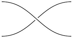
In pictures the distributive law can be drawn as one string “jumping over” another

and the axioms just say that the monoidal structures (dots) pass through those crossings:

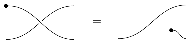
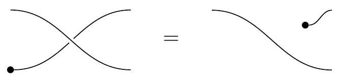
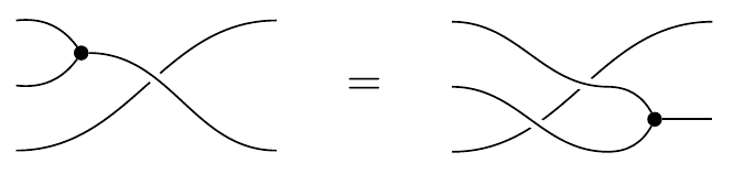
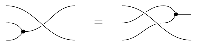
The wire that does the jumping is shown as unbroken, whereas the wire that got jumped is shown as broken. This graphical notation fits with the jump law: the jumper is left intact and unmodified, whereas the jumpee is left modified by the jumper. Similarly the textual notation of writing (A,B)\mapsto(B^A,A) also fits nicely with the jump law: we see the jumper A is unmodified, whereas the jumpee B is modified by A jumping over it.

One way to understand the fact that \nabla goes from u\triangleleft u to u\otimes u is that we start with a dependent type, e.g. (T : \mathrm{Type}, (t : T)\mapsto (U_t : \mathrm{Type}), and goes to two independent types, namely \prod_{t : T}U_t : \mathrm{Type} and T : \mathrm{Type}.

So in some sense, \Pi can be thought of as the second string, after it’s been jumped over, the B^A or \prod_{a\in A}B(a) thing; more precisely, it is either map u\triangleleft u\triangleleft 1\to u\triangleleft 1 in the following commutative diagram \begin{CD} u\triangleleft u\triangleleft\,1 @>\nabla\triangleleft\,1>> (u\otimes u)(1) @= u(1)\times u(1) \\@. @VVV @VVV \\@. u\triangleleft u\triangleleft\,1 @>\nabla\triangleleft\,1>> u(1) \end{CD}

From the distributive law, we can derive the fact that \Pi is a u-algebra, which is part of Awodey’s definition.

Claim. The map \Pi\colon u(u(1))\to u(1) gives u(1) the structure of a u-algebra.

Proof: Let X:=u(1); we need to show that \Pi\colon u(X)\to X makes X an algebra of the monad u, i.e. X\to u(X)\to X is the identity on X and the two maps u(u(X))\to X agree. Since \Pi is just u\triangleleft 1, both can be shown entirely with string diagrams.

But examples will help the most in understanding this. The most instructive in terms (no pun intended!) of dependent types are Examples 3.3 and 3.4 below. But first we give a few warmups.

3 Examples

3.1 Monoids with exponentiation

Let (M,e,\star) be a monoid, and suppose there is an operation (\,\hat{}\,)\colon M\times M\to M, denoted (m,n)\mapsto m^n, satisfying the following properties for all m,m_1,m_2,m_3\in M: \begin{aligned} m^e &= m \\ e^m &= e \\ (m_2\star m_3)^{m_1} &= m_2^{m_1}\star m_3^{m_1} \\ m_3^{(m_1\star m_2)} &= (m_3^{m_2})^{m_1} \end{aligned} We refer to this structure as a monoid with exponentiation.

As mentioned above, the multiplicative monoid (\mathbb{N},e,\star) of natural numbers has an exponential structure, e.g. 3^4=81. Thus by the above work we can define a jump structure on it.

Now note that M\mathcal{y} is itself a polynomial, since M is a set; it’s a linear polynomial, and maps between linear polynomials are just maps of sets \mathbf{Poly}(A\mathcal{y}, B\mathcal{y}) \cong \mathbf{Set}(A,B). Note also that (M\mathcal{y})\triangleleft(M\mathcal{y})\cong(M\mathcal{y})\otimes(M\mathcal{y})\cong(M\times M)\mathcal{y}.

The polynomial M\mathcal{y} has a (Cartesian) monad structure, where the unit is e\colon \mathcal{y}\to M\mathcal{y} and the multiplication is \star\colon (M\mathcal{y})\triangleleft(M\mathcal{y})\to M\mathcal{y}. Now we can use the exponential structure of M to get a distributive structure on M\mathcal{y} that satisfies the jump law. First we need a candidate map M\mathcal{y}\triangleleft M\mathcal{y}\to M\mathcal{y}\otimes M\mathcal{y}, i.e. a map M\times M\to M\times M. Let’s use (m,n)\mapsto (n^m, m). The jump law holds because the first variable of (m,n) equals the second variable of (n^m,m), and the four distributive laws require the following equations between ordered pairs: \begin{aligned} (m^e,e) &= (m,e) \\ (e^m,m) &= (e,m) \\ ((m_2\star m_3)^{m_1},m_1) &= (m_2^{m_1}\star m_3^{m_1},m_1) \\ (m_3^{(m_1\star m_2)},m_1\star m_2) &= ((m_3^{m_2})^{m_1},m_1\star m_2) \end{aligned} all of which we have by assumption. Our definition of \Pi in terms of \nabla says that \Pi(m,n):= n^m, which is the exponentiation operation we started with.

3.2 Conjugation in group theory

Let (G,e,\star) be a group. Then we can consider it as a monoid and define an exponential structure on it by conjugation: h^g:=ghg^{-1} The required equations are \begin{aligned} ege^{-1} &= g \\ geg^{-1} &= e \\ g(hi)g^{-1} &= (ghg^{-1})(gig^{-1}) \\ (gh)i(gh)^{-1} &= g(hih^{-1})g^{-1} \end{aligned} Our definition of \Pi in terms of \nabla says that \Pi(g,h)=ghg^{-1}, which is the conjugation.

Let’s change gears a bit. The following example on lists is good intuition for the example on natural models. Roughly speaking, it’s talking about the universe of finite sets, encoded as natural numbers.

3.3 List monad

Consider the functor \mathrm{List}\colon \mathbf{Set}\to \mathbf{Set}, which sends X\mapsto\sum_{N\in\mathbb{N}}X^N We denote the pair (N,f) where f\colon \prod_{1\leq n\leq N}\to X by [f(1),f(2),...,f(N)].

\mathrm{List} has a well-known monad structure, where we take the unit y\to \mathrm{List} to be the “singleton” map X\to \mathrm{List}(X), i.e. that given by x\mapsto [x], and we take the multiplication to be the “concatenate” map sending (M,(N,f)) where M\in\mathbb{N} and N\colon \prod_{1\leq m\leq M}\to \mathbb{N} and f\colon\prod_{1\leq m\leq M}\to\prod_{1\leq n\leq (N m)}\to X to (\sum_{1\leq m\leq M}N m,(m,n)\mapsto X m n). The list monad is Cartesian.

For our distributive structure, we need to take a list of lists and return another list of lists. The intuition can be obtained from the following example: the distributive law will transform the thing on the left to the thing on the right: [[1,2],[3,4,5]] \mapsto [[1,3],[1,4],[1,5],[2,3],[2,4],[2,5]]. Do you see how in the right-hand list-of-lists, the number of elements in each sublist is always 2? This means that the interior list length is independent of what entry it’s in, unlike the left-hand list-of-lists, where the first entry is shorter than the second. The distributive law will eventually tell us that if we sum-then-multiply the first list-of-lists, the result is equal to what we get if we multiply-then-sum the second list-of-lists. To check, we get 3*12 on the left and 3+4+5+6+8+10 on the right; success!

Ok, so what exactly is the distributive structure \mathrm{List}\triangleleft \mathrm{List}\to \mathrm{List}\triangleleft \mathrm{List}? It is given by (M,N,f)\mapsto \left(\prod_{m\in M}N\ m, M, (n, m)\mapsto f\ m\ (n\ m)\right). Our definition of \Pi in terms of \nabla says that \Pi is product of sets (M\in\mathbb{N},N\colon M\to\mathbb{N})\mapsto\prod_{m\in M} N\ m.

3.4 Natural models with sum and product types

The definition of jump structure was designed to extract part of what we see in Awodey’s notion of natural models. In particular, he gives a Cartesian polynomial monad u:=\sum_{A\in U}\mathcal{y}^{[A]}, or as we prefer to write it u:=\sum_{A\in u(1)}\mathcal{y}^{u[A]}. Its universe’s positions are called types and the directions at a type A\in u(1) are called terms of type A, denoted a\in u[A]. The monad structure (u,\top,\Sigma) gives both the unit type and the dependent sum structure.

Steve also requires that u(1) have an additional u-algebra structure, meaning we need a map u\triangleleft u(1)\to u(1), to serve as the \Pi operation. This is where the jump structure \nabla\colon u\triangleleft u\to u\triangleleft u comes in; we define \Pi by u\triangleleft u\triangleleft 1 \xrightarrow{\nabla\triangleleft\ 1} u\triangleleft u\triangleleft 1 \xrightarrow{u\triangleleft\ !} u\triangleleft 1 There are four distributivity laws, but only two laws necessary for \Pi to give u(1) the structure of a u-algebra. The reason is that \Pi basically discards the second variable (see the “u\triangleleft !” ?). But the two relevant laws say this: \Pi(A,\top)=\top \qquad\text{and}\qquad \Pi(A,\Sigma(B, C)) = \Sigma(\Pi(A, B),C) for any A\in u(1), B\in\prod_{a\in u[A]}u(1), and C\in\prod_{a\in u[A]}\prod_{b\in B(a)}u(1).

4 Discussion

I’m guessing that jump monads are not really where this story is supposed to end up. They are interesting, but there are several things missing. Let’s first discuss some extra structures we might want to impose.

4.1 Additional structures

Finite coproducts. A jump monad has a \Sigma operation, but that doesn’t mean we can form finite coproducts; it just means we can form A-indexed coproducts for any A\in u(1). To get 0-ary and 2-ary coproducts, we’d need Cartesian maps \bot\colon 1\to u and \mathbb{B}\colon \mathcal{y}^2\to u which would pick out types that we could call the empty type and the Boolean type. Then we could define 0-ary and 2-ary coproducts to be given by 1\triangleleft u\xrightarrow{\bot\triangleleft\ u}u\triangleleft u\xrightarrow{\Sigma}u \qquad\text{and}\qquad \mathcal{y}^2\triangleleft u\xrightarrow{\mathbb{B}\triangleleft\ u}u\triangleleft u\xrightarrow{\Sigma}u. Now 1\triangleleft u\cong 1 and \mathcal{y}^2\triangleleft u\cong u\times u, so we could ask that the maps \bot\colon 1\to u \qquad\text{and}\qquad (+)\colon u\times u\to u satisfy the monoid laws; then we would have finite coproducts in our type theory. This also works for our List example, but unfortunately it does not work for our example of monoids with exponential structure because there is no Cartesian map \mathcal{y}^2\to M\mathcal{y}; it would be quite cool if we could somehow get the axioms for a rig with exponential structure this way.

Here’s another weird thing. The map \mathcal{y}^2\to u also allows us to form binary products via \mathcal{y}^2\triangleleft u(1)\xrightarrow{\mathbb{B}\triangleleft u(1)} u\triangleleft u(1)\xrightarrow{\nabla(1)} u\triangleleft u(1)\xrightarrow{u\triangleleft\ !} u(1) This is just using \Pi to define binary products, i.e. saying that A_1\times A_2 is \prod_{i\in\mathbb{B}}A_i. But we already had what’s arguably a nicer way to form binary products, namely u\otimes u\xrightarrow{\mathrm{indep}}u\triangleleft u\xrightarrow{\Sigma} u Now (u\otimes u)(1)\cong(u\triangleleft u)(1)\cong (u\times u)(1)\cong \mathcal{y}^2\triangleleft u(1), so we can ask these two different approaches give the same answer, after we plug 1 into the second formulation. But the connection between them doesn’t seem like the most elegant formulation, does it?

4.2 Additional “internal” condition for jump structure

The last thing I want to mention is that there is an additional condition that we might want to encode about the jump structure. Here’s the informal way to say it.

Given a type A\in u(1) and a dependent type B(a)\in u(1) for each a\in u[A], the jump structure gives us two independent types, \Pi_{a\in A}B(a) and A, and a way to take terms (b,a) of the latter and return terms (a, b(a)) of the former. But there’s an additional thing we might want, namely the evaluation map (\Pi_{a\in A}B(a))\times A\to B. Using all our structures, we seem to want a 2-arrow as shown here:

In string diagrams, where we draw the distributivity by having one string jump over another and the monad structure as a monoid operation, this e map looks like a kind of “untwisting” operation. The string diagram syntax then suggests four laws that e should satisfy. Since I don’t have good drawing tools for this blog, I’ll use text notation instead. First let’s give a notation for e itself: e_{A,B}\colon B^AA\Rightarrow AB the idea being that given elements b : \Pi_{a\in A}B(a) and a : A, we get an element (a, b(a)) : \Sigma_{a\in A}B(a). Now the four laws say: \begin{CD} A @= A \\@| @| \\A^{1}1 @>>e_{A,1}> 1A \end{CD} \qquad \begin{CD} A @= A \\@| @| \\1^{A}A @>>e_{1,A}> A1 \end{CD} and \begin{CD} (C^B)^{A}AB @>e_{A,C^B}B>> AC^{B}B \\@| @VVAe_{B,C}V \\C^{(AB)}AB @>>e_{AB,C}> ABC \end{CD} Again, these four laws look quite natural in the string diagram calculus.

But hold on a minute! Where is this \Downarrow map that we’ve been calling e supposed to live exactly? We could say that it lives in the full internal subcategory defined above. So to say this part, we need to leave the pure polynomial world and use this full internal subcategory idea. Perhaps this is fine, but I’m not completely happy with it.

4.3 Conclusion

The reason all this is a blog and not a paper is that it is a collection of thoughts that is relatively stable and may be useful to someone, but it leaves room for improvement. I do think it is already somewhat interesting. For example, I’d never really seen a self-distributivity law u\triangleleft u\to u\triangleleft u in practice before. And though I found it by trying to impose the distributivity law between \Sigma and \Pi, as suggested by André Joyal’s question to Steve, it was quite surprising that this law defines \Pi, at least at the type level. Finally, the fact that this notion is exemplified by group conjugation and exponentiation in monoids means that it’s pointing to something beyond the one example that motivated it.