Creating new categories from old: Selection categories
polynomial functors
Abstract
In this short post, I’ll describe a way of creating new categories from old. It reminds me of a ‘particle filter’ or ‘natural selection’. This method comes from the theory of polynomial functors, but I’ll confine all the technical details to a single section, so you don’t need to know anything about polynomial functors to read this post.
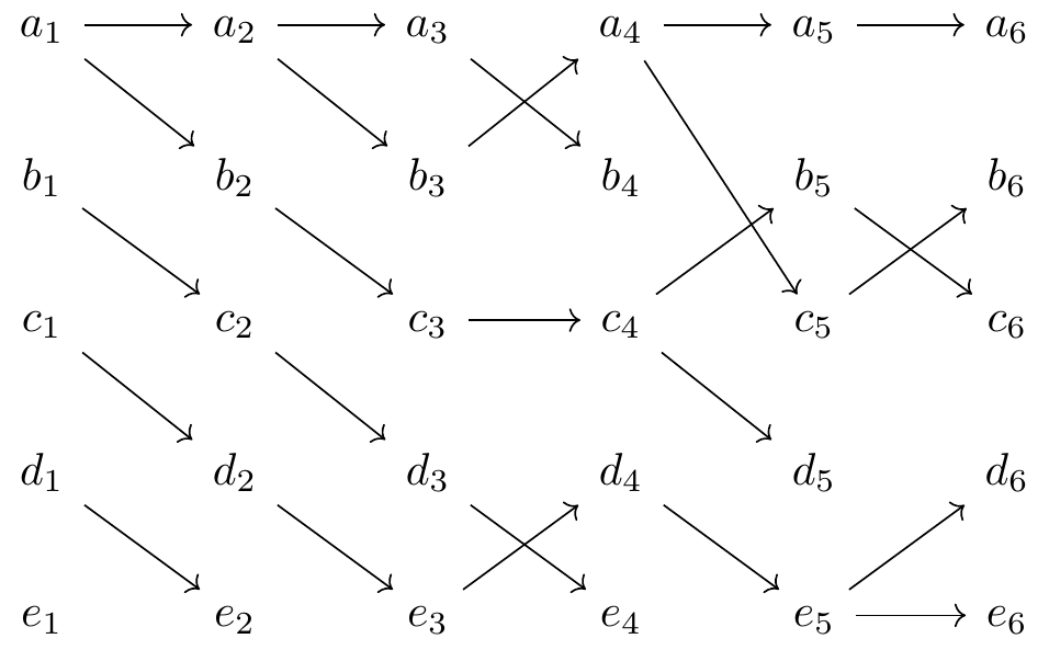
TL;DR: The following picture captures the entire idea:
Here, each of the a_1,a_2,\ldots,e_6 are objects in the original category, and every arrow is an arrow in the original category. In the associated select-5 category, an object is a whole column (e.g. (a_3,b_3,c_3,d_3,e_3) is one object) and a morphism between them is a column of arrows as shown. The composite is the obvious thing you get by “path following”, e.g.

In some sense, it looks like a_1 and c_1 were the most “successful” of the initial cohort, since at stage 6, every object is “descended” from one of those two.
1 Introduction
There are many known ways to get new categories from old. Given a category C, you can take its opposite, you can adjoin a terminal object, you can take the coproduct or product of it with itself, etc. In this post, I’ll tell you about a new such category-generating machine.
For today, I’ll call the result “selection categories”. The reason for the name might be clear from the example at the top: it was as though we had a situation with a limited number of slots—in that case, five—and in every column we chose to extend only some of the previous objects. In the end, we have five things, but they are “descended from” only two of the original five. However, it is important to note that nothing about “nature” is making the choices here—the category contains all possible choices—so I hope the name and metaphor aren’t too misleading. I won’t discuss selection in the sense of evolution any further; instead, I’ll just describe the mathematics.
2 Input data
In order to run this construction, you need two things.
- the category C you want to run it on, and
- a polynomial p in one variable (I like to use y for my variable) whose coefficients are all natural numbers (or more generally, sets).
In the above case I used the polynomial y^5, but our second example will be y^5+y^3. Let’s write p=\sum_{i\in I}y^{p[i]}, and refer to each i\in I as a tag and the set p[i] as the slot-count for tag i. The reason is that the p[i]’s tell you the legal numbers of slots that our columns are allowed to have in them. We also think of p[i] as a set, the set of slots. The introductory example had only one tag with slot-count 5; instead of a number, we could think of this tag as representing a column, a set of five elements, (a,b,c,d,e).
Once we have our slot-counts, we want to actually select objects from our category to fill those slots. Just as we refered to y^5 as the “select-5” polynomial, let’s refer to y^5+y^3 as the select-5 or select-3 polynomial. If more than one summand has the same exponent, then we have to tag them seperately, e.g. we could refer to y^5+2y^3 as the select-5 or select-3-tag-A or select-3-tag-B polynomial.
3 The selection category on p
Given a polynomial p=\sum_{i\in I}y^{p[i]} and a category C, we’re ready to say what the objects and morphisms in our new category are. In my own personal work I like to denote this new category \left[\begin{matrix} p\\ p\triangleleft C \end{matrix}\right] because it comes from a certain “coclosure” operation in \mathbf{Poly} that generalizes lenses from functional programming. But again, you can ignore that for today.
An object in this new category \left[\begin{smallmatrix} p\\ p\triangleleft C \end{smallmatrix}\right] is a pair (i, c), where i\in I is a tag and c\in\mathsf{Ob}(C)^{p[i]} is a selection of p[i]-many objects in C. That is, we have filled our slot-count with objects; let’s call c a cohort. So a column like (a_3,b_3,c_3,d_3,e_3) in our original example constitutes one object—one cohort—in \left[\begin{smallmatrix}y^5\\y^5\triangleleft C\end{smallmatrix}\right].
A morphism from (i,c) to (i',c') is a pair (f,g) where f\colon \{1,\ldots,p[i']\}\to\{1,\ldots,p[i]\} is a backwards-facing function between slot sets, and where g assigns to each slot s\in \{1,\ldots,p[i']\} a morphism in C from c_{fs} to c_s'. So every slot in cohort c' receives a morphism from some choice of slot in cohort c. Take another look at the example to make sense of that.
Every map in \left[\begin{smallmatrix}p\\p\triangleleft C \end{smallmatrix}\right] can be uniquely factored as a composite of two simpler kinds of map. The first factor will be a pure selection (no “aging”), meaning that the tags and slots can change, but all the arrows are identities. The second factor will be a pure “aging” (no selection), meaning that the tags don’t change and it’s a “straight-across” map, but the arrows can be anything you want.

4 Examples
We promised to do y^5+y^3 next, i.e. to consider the category \left[\begin{smallmatrix} y^5+y^3\\ (y^5+y^3)\triangleleft C \end{smallmatrix}\right]. Rather than just repeating the definition in this case, we’ll just draw a picture of five composable morphisms
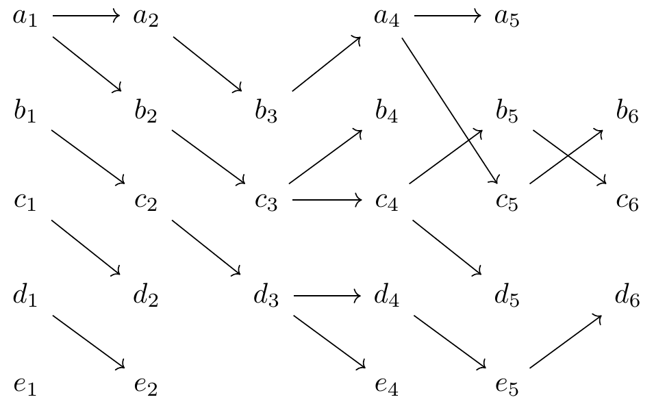
So the number of slots varies, but the idea is identical.
The select-1 or select-0 from C category \left[\begin{smallmatrix}y+1\\(y+1)\triangleleft C\end{smallmatrix}\right] corresponding to the polynomial y+1, is given by adding a free terminal object to C. That is, an object is either an object of C or an empty column, which we’ll call nothing. A morphism between two objects from C is just a morphism from C. There is a unique morphism from anything to nothing, and the only map out of nothing is the identity.
Repeats don’t do too much. For example 3y would just give you three different tags for objects in C, that you can freely move between. That is, \left[\begin{smallmatrix}3y\\(3y)\triangleleft C\end{smallmatrix}\right] is just the product of C and a “co-discrete category” of size 3 (where the co-discrete category on A has A-many objects and a unique morphism between any two).
As another example, y+3 would adjoin a whole co-discrete category of size 3 as a terminal subcategory. You can move around in C as much as you want, and then eventually go to three different sorts of nothing, which you can move freely between forever.
Another fun one: if you take C=1 to be the one-morphism category and you take p=y^2+y, then the resulting category \left[\begin{smallmatrix}y^2+y\\(y^2+y)\triangleleft 1\end{smallmatrix}\right] is the indexing category for symmetric reflexive graphs. It has two objects, say V and E for “vertex and edge”. And other than identities it has two maps E\rightrightarrows V for “source and target”, a map V\to E for “identity edge”, and a map E\to E for “dual edge”.
That about does it! Next I’ll give a technical section for interested readers, but for the rest of you, I suggest you skip it and go right to the last section, where I describe a sequence of important categories that arises from this construction.
5 Technical stuff
For any polynomial p, the construction \left[\begin{smallmatrix}p\\p\triangleleft -\end{smallmatrix}\right] is functorial; in fact it sends bijective-on-objects functors to bijective-on-objects functors and sends fully faithful functors to fully faithful functors. It is in fact an oplax framed functor from \mathbb{C}\mathbf{at}^\sharp to itself, where \mathbb{C}\mathbf{at}^\sharp is the framed bicategory of comonoids and comodules in \mathbf{Poly}.
Given any polynomials p,q and category C, there is a canonical profunctor from \left[\begin{smallmatrix}p\\ p\triangleleft C\end{smallmatrix}\right] to \left[\begin{smallmatrix}q\\q\triangleleft C\end{smallmatrix}\right]. It assigns a set to any pair ((i,c),(j,d)) of objects, where c\in C^{p[i]} and d\in C^{q[j]}, namely: it assigns the set of pairs (f,g) where f\colon q[j]\to p[i] is a backwards-facing function and g assigns to each slot s\in \{1,\ldots,q[j]\} a morphism in C from c_{fs} to d_s. Very reasonable, right? And in the presence of a cartesian map of polynomials p\to q, the above profunctor arises as the pullback along a fully faithful functor \left[\begin{smallmatrix}p\\p\triangleleft C\end{smallmatrix}\right]\to\left[\begin{smallmatrix}q\\q\triangleleft C\end{smallmatrix}\right].
One last kind of interesting technical thing. For any p,q there is a bijective-on-objects functor from \left[\begin{smallmatrix}p\\p\triangleleft C\end{smallmatrix}\right]+\left[\begin{smallmatrix}q\\q\triangleleft C\end{smallmatrix}\right] to \left[\begin{smallmatrix}p+q\\(p+q)\triangleleft C\end{smallmatrix}\right]. For example, taking p=P and q=Q to be sets, consider the complete graph K_P on P vertices and the complete graph K_Q on Q vertices, but think of them as categories (contractible groupoids). Their disjoint union K_P+K_Q is not the complete graph K_{P+Q} on P+Q-vertices, but it is still a category and there is a bijective-on-objects functor K_P+K_Q\to K_{P+Q} between them.
6 One last trick
Consider the list polynomial u=1+y+y^2+y^3+\cdots. The functor C\mapsto\left[\begin{smallmatrix}u\\u\triangleleft C\end{smallmatrix}\right] is one that my colleague Evan might call the category of “product diagrams in C”. But I’m interested in a slight variant of this, namely \left[\begin{smallmatrix}u\\u\triangleleft -\end{smallmatrix}\right]^{\text{op}}.
Suppose you apply this functor repeatedly, starting from the empty category 0; what do you get?
Applying it once you get \left[\begin{smallmatrix}u\\u\triangleleft 0\end{smallmatrix}\right]^{\text{op}}=1, i.e. the one object category, because the only way to write down N objects from the empty category is if N=0.
Ok, we have 0, 1, what’s next? We calculate that the next iteration \left[\begin{smallmatrix}u\\u\triangleleft 1\end{smallmatrix}\right]^{\text{op}}\simeq\mathbf{FinSet} is a skeleton of finite sets. Indeed, just write down columns of any size (all with “1” filling every slot), and identity maps backwards between them. Then, since we’re supposed to take an opposite, flip the direction of the arrows so the maps go forwards. Nothing’s going on except the number of dots, so you see we just get the category of finite sets and maps between them!
Ok, so we now have 0, 1, \mathbf{FinSet}. What’s next? I’ll save that for the curious reader. Feel free to post it in the comments below if you figure it out!