Recursive Types via Domain Theory

Abstract

Functional programming languages often include recursive types, allowing programmers to define types satisfying a given isomorphism. Such types cannot all be interpreted as sets, but they can be understood using domain theory. We consolidate and present foundational techniques in domain theory to understand eager programming languages with recursive types from a categorical perspective. We define a category of domains with finite coproducts, a symmetric monoidal closed structure for eager products and functions, and least solutions of recursive domain equations, whose objects are retracts of a universal space and whose morphisms are continuous with respect to a topology of approximations.

1 Introduction

When writing code, it is common to use recursive types to represent data structures. As a simple example, one might want a type representing the natural numbers. The type of natural numbers can be characterized as the least type such that N \cong 1 + N; we will refer to constraints of the form X \cong F(X) as domain equations. In ML-style pseudocode, a least (i.e., inductive) solution to this type equation may be defined as follows:

datatype N = Fold of 1 + N
val unfold = fn (Fold x) => x

Here, Fold : 1 + N -> N is the name of the constructor. Via pattern matching, we define its inverse, unfold : N -> 1 + N. Sometimes, types are informally thought of as sets; this type N is thought of as the set \mathbb{N} of natural numbers.

For a more unusual example, non-total programming languages (such as Standard ML, OCaml, and Haskell) allow the following pseudocode:

datatype C = Fold of C -> 2
val unfold = fn (Fold x) => x

This defines a type C that is isomorphic to the “function space” from C to 2! In this case, set-oriented reasoning breaks down: by Cantor’s Theorem, there is no set C isomorphic to its power set, 2^C. However, types of this form are very powerful, underpinning unbounded recursion. For example, using C, we may write a diverging (i.e., “infinitely looping”) program by applying an element c : C to itself (up to the given isomorphism):

(* unroll : C -> 2 *)
val unroll = fn (c : C) => (unfold c) c

(* val diverge : 2 *)
val diverge = unroll (Fold unroll)

This example begins to demonstrate the power granted by recursive types.¹

In order to give a categorical account of languages with such unusual type isomorphisms, we must find a suitable category to work in. The category of sets has too many morphisms between each pair of objects, which prevents us from defining types like C; thus, we will work in a subcategory of domains that imposes further topological restrictions. In particular, this subcategory will be capable of expressing that some programs may be partially defined (i.e., diverge sometimes).

To model a reasonable eager functional programming language, we will ensure that this subcategory has finite coproducts, a symmetric monoidal closed structure for eager products and functions, and least fixed points of domain equations. We will not give a formal interpretation of a programming language into the category, but we will treat its objects as types and its morphisms as programs in the standard way.

2 Directed-Complete Partial Orders

We begin by defining a subcategory of \mathbf{Poset}, called \mathbf{DCPO}, whose objects will ultimately correspond to types. Objects of \mathbf{DCPO} will be posets with particular sensible least upper bounds.

Definition

Let X = (U X, \le_X) be a poset. Say X is directed iff every finite subset of U X has an upper bound with respect to the \le_X ordering.

Corollary

Every directed set X is nonempty, since the empty set is finite and its upper bound must therefore exist in X.

Definition

A directed-complete partial order (DCPO) is a poset D = (U D, \le_D) such that all directed subsets X \subseteq U D have a least upper bound, \bigsqcup_D X, with respect to the \le_D ordering.

We will understand each type as a DCPO D, where the elements of a type are simply the elements of UD. For x, y \in UD, we understand x \le_D y as “x is at most as defined as y”. For example, a diverging computation (i.e., “infinite loop”) will be less defined than a result value.

Example

Every discrete poset (A, =) is a DCPO, the discrete DCPO. The only directed subsets of A are singleton sets of the form \{{a}\} for a \in A, which have least upper bound a. For readability, we will abbreviate DCPO (A, =) as A.

Discrete DCPOs will correspond to positive types. For example, 2 = \{{0, 1}\} will correspond to the Boolean type, the type type with two values.

Example

Consider the following poset, \mathbb{T}:

Since every directed subset has a least upper bound, \mathbb{T} is a DCPO. Note, however, that not every subset has a least upper bound: the non-directed subset \{{0, 1}\} has no upper bound at all.

\mathbb{T} will be the type of computations of a Boolean value, which can be in \{{0, 1}\} or can be a computation \bullet that diverges. Divergence is less defined than any Boolean value, but both Boolean values are on equal footing when it comes to definedness.

Well-behaved functions between DCPOs, known as Scott-continuous functions, should preserve the DCPO structure.

Definition

Let D and E be DCPOs. Then, a Scott-continuous function f : D \to E is a (monotone) function D \to E that preserves directed suprema; i.e., f(\bigsqcup_D X) = \bigsqcup_E f(X) for all directed X \subseteq U D.

Remark

Continuity will be used here to approximate computability. In particular, if f : D \to E is continuous, we may think about f as a computable function from type D to type E.

We may now define the category \mathbf{DCPO} of DCPOs in the obvious way.

Definition

\mathbf{DCPO} is the category with DCPOs as objects and Scott-continuous functions as morphisms.

Remark

Each DCPO D has an associated topology (the Scott topology), built from continuous maps from D into the DCPO of truth values \{{\bot \le \top}\}, for which the given notion of Scott continuity is the same as topological continuity. Therefore, \mathbf{DCPO} is a full subcategory of \mathbf{Top}, the category of topological spaces.

The category \mathbf{DCPO} has plenty of structure, which will let us understand sum, eager product, and function types.

Theorem

\mathbf{DCPO} is bicartesian closed. Products and coproducts are inherited from \mathbf{Poset}, and the exponential D \to E is the DCPO consisting of all Scott-continuous functions from D to E, ordered pointwise. (Abramsky and Jung 1994)

3 Diverging Computations and Partial Functions

As discussed in the introduction, in a programming language with recursive types, a computation may diverge (i.e., “infinitely loop”). While a value of Boolean type must be either 0 or 1, a computation of a Boolean may be a value 0 or 1, or it may diverge. Thus, for each DCPO D of values, we will define a corresponding DCPO {D}_\bot of potentially-diverging computations.

Definition

Let D be a DCPO. The lifting of D, written {D}_\bot, is a DCPO consisting of D with a fresh least element adjoined. Concretely: \begin{aligned} U({D}_\bot) &\triangleq\{{\bot}\} + D \\ x \le_{{D}_\bot} y &\triangleq(x = \bot) \lor (x \le_D y) \end{aligned}

Remark

The DCPO \mathbb{T} is simply {2}_\bot.

In an eager functional programming language, a function evaluates its definition and performs any suspended behaviors when applied to an argument. For example, values of the thunk type unit -> t are computations of type t, which may diverge when the function is applied to the unique value of type unit (typically written ()). If t corresponds to a DCPO D, we will see that unit -> t corresponds to {D}_\bot. We may understand this phenomenon by viewing partiality as an effect, embodied by the lift monad.

Definition

The lift monad {(-)}_\bot : \mathbf{DCPO}\to \mathbf{DCPO} is the functor that sends a DCPO D to {D}_\bot.

Remark

The lift monad is similar to the common maybe monad, (-) + 1, in that it also adjoins a fresh new element. However, \bot is less than all existing elements, whereas the element adjoined by (-) + 1 is incomparable to all existing elements. This expresses the subtle difference between the recoverable failure effect and partiality.

For example, it is trivial to define a function of type D + 1 \to 2 that computes whether its input “failed”. However, it is impossible to write a function {D}_\bot \to 2 that computes whether its input “failed” (was \bot); such a function would not even be monotone. Informally, this corresponds to the undecidability of the Halting problem, which says that it is impossible to write a program that decides whether its input computation terminates or diverges.

Now, we may work in the Kleisli category of this monad, following the typical development by Moggi (1991) of categorical models of effectful eager functional programming languages.

Definition

The Kleisli category of the lift monad, {\mathbf{DCPO}_\bot}, has the same objects as \mathbf{DCPO}. However, a morphism D \to E in {\mathbf{DCPO}_\bot} is a morphism D \to {E}_\bot in \mathbf{DCPO}, a partial function continuous on a Scott-closed subset of D into E.

Remark

The category {\mathbf{DCPO}_\bot} is equivalent to the subcategory of \mathbf{DCPO} where an object is a pointed DCPO (i.e., a DCPO with a least element) and morphisms are required to be strict (i.e., least element preserving). This alternative presentation is common in the literature (Plotkin 1978), but we find the Kleisli category presentation more elegant: it aligns with the operational semantics of an eager functional programming language (where divergence is not legal to substitute as an input) and the usual semantics for monadic effects (Moggi 1991). Explanation of the significance behind this perspective is explained further by Levy (2003).

Theorem

Since \mathbf{DCPO} has coproducts, so too does the Kleisli category {\mathbf{DCPO}_\bot}.

Although \mathbf{DCPO} has products, the object D \times E from \mathbf{DCPO} is not a categorical product in {\mathbf{DCPO}_\bot}: the presence of the partiality effect breaks the existence condition of the universal property for products.² Although \mathbf{DCPO} products are not categorical products in {\mathbf{DCPO}_\bot}, they will still be useful for understanding eager product types.

Theorem

The categorical product in \mathbf{DCPO} is a symmetric monoidal product in {\mathbf{DCPO}_\bot}, written (\otimes, I).

{\mathbf{DCPO}_\bot} is also closed with respect to this monoidal structure. Let the internal hom D \multimap E be defined as D \Rightarrow_\mathbf{DCPO}{E}_\bot. Then, (-) \otimes D is left adjoint to D \multimap(-).

We will understand eager product and function types as \otimes and \multimap, respectively.

4 Domains as Retracts of a Universal Space

We may now define a category of domains in which we can solve domain equations, which will be a subcategory of {\mathbf{DCPO}_\bot}. Informally, a domain will be an DCPO whose elements can be encoded as sequences of bits.

Definition

Let \mathbb{U} be the DCPO \mathbb{N}\multimap 2, partial functions from \mathbb{N} to 2.³ In other words, the elements of \mathbb{U} are the infinite streams of elements of {2}_\bot.

We will call \mathbb{U} the universal domain.

We will sometimes write elements of \mathbb{U} as infinite streams s of the form ({x}, {s'}), where x \in {2}_\bot and s' is another infinite stream, in place of a function i \mapsto \begin{cases} x & i = 0 \\ s'(i - 1) & i > 0. \end{cases} Additionally, to disambiguate between the bottom element available from the Kleisli category and the bottom element of {2}_\bot, we will refer to the latter as \bullet (as in \mathbb{T}).

A domain will be a DCPO that can be encoded in the universal space \mathbb{U}. We formalize this encoding property using the categorical notion of retract.

Definition

Let A and B be objects in a category. A is a retract of B if there exist maps i_{A} : A \to B and r_{A} : B \to A such that i_{A};r_{A} = \text{id}_{A}, where ; denotes forward composition.

Call i_{A} the encoder (or section) and r_{A} the decoder (or retraction).

With this definition in hand, we may define “domain” in this setting.

Definition

A DCPO D is a domain iff it is a retract of \mathbb{U} in {\mathbf{DCPO}_\bot}.

In other words, a domain is a DCPO that can be faithfully encoded into \mathbb{U}.

Definition

Define \mathbf{Dom} to be the full subcategory of {\mathbf{DCPO}_\bot} consisting of domains.

This category \mathbf{Dom} is what we were originally looking for: recursive types will make sense within \mathbf{Dom}. Let us now consider some examples of domains.

Example

The discrete DCPO 2 of Boolean values is a domain, with encoder and decoder defined by: \begin{aligned} i_{2} &\triangleq x \mapsto ({x}, {\overline{\bullet}}) \\ r_{2} &\triangleq({x}, {s}) \mapsto x \end{aligned} where \overline{\bullet} is the infinite stream of \bullet\in {2}_\bot. Clearly, i_{2};r_{2} = \text{id}_{2}. In other words, a Boolean value is encoded as a single bit, the first in the infinite stream (followed by \bullet values).

When working with coproducts, we write [-, -] for copairing, \iota_1 for the left injection, and \iota_2 for the right injection.

Example

If D and E are domains, then the coproduct D + E in {\mathbf{DCPO}_\bot} is a domain. Its encoder and decoder defined by: \begin{aligned} i_{D + E} &\triangleq[d \mapsto ({0}, {i_{D}d}), e \mapsto ({1}, {i_{E}e})] \\ r_{D + E} &\triangleq({x}, {s}) \mapsto \ \begin{cases} \iota_1(r_{D}s) &\text{if } x = 0 \\ \iota_2(r_{E}s) &\text{if } x = 1 \\ \bot &\text{if } x = \bullet \end{cases} \end{aligned} Informally, this encodes an element of D + E by using the first bit as a “tag bit” and encoding the data in the remaining bits.

The nullary coproduct 0 is a domain, as well, with i_{0} \triangleq¡ and r_{0} \triangleq s \mapsto \bot.

Example

If D and E are domains, then the monoidal (“eager”) product D \otimes E in {\mathbf{DCPO}_\bot} is a domain. Its encoder and decoder defined by: \begin{aligned} i_{D \otimes E} &\triangleq\langle d, e \rangle \mapsto (h^{-1};[i_{D}d, i_{E}e]) \\ r_{D \otimes E} &\triangleq s \mapsto \langle r_{D}(\iota_1;h;s), r_{E}(\iota_2;h;s) \rangle \end{aligned} where h : \mathbb{N}+ \mathbb{N}\to \mathbb{N} is a standard isomorphism (e.g., interleaving via evens and odds). Informally, this encodes an element of D \otimes E by encoding its components and interleaving their bit representations.

The nullary monoidal product I = \{{\star}\} is a domain, as well, with i_{I} \triangleq\star \mapsto \overline{\bullet} and r_{I} \triangleq s \mapsto \star.

Example

If D and E are domains, then the internal hom D \multimap E \triangleq D \Rightarrow_\mathbf{DCPO}{E}_\bot in {\mathbf{DCPO}_\bot} is a domain.

We elide the details of the construction here, although they are described in full by Plotkin (1978). Informally, an element of D \multimap E is encoded as its “graph”, expressing all of its input-output pairs as a bit stream. Details about Scott’s model, a similar construction, are given in a recent blog post by my co-mentee.

5 Recursive Types

We will now see that the category \mathbf{Dom} has least fixed point solutions to domain equations.

Definition

Say encoding/decoding pair (i_{} : D \to E,\ r_{} : E \to D) is an embedding-projection pair if r_{};i_{} \le \text{id}_{E}. Define {\mathbf{Dom}_\triangleleft} to be the wide subcategory of \mathbf{Dom} where a morphism D \to_{\mathbf{Dom}_\triangleleft}E is an embedding-projection pair, written {D} \triangleleft {E}.

Theorem

In {\mathbf{Dom}_\triangleleft}, every \omega-chain has a colimit. (Smyth and Plotkin 1982)

In other words, every diagram of the following shape has a colimit:

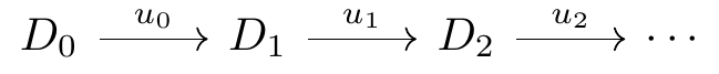
Expressed in \mathbf{Dom}:

Lemma

{\mathbf{Dom}_\triangleleft} inherits coproducts and monoidal products from \mathbf{Dom}.

Corollary

Every endofunctor F : {\mathbf{Dom}_\triangleleft}\to {\mathbf{Dom}_\triangleleft} has a least fixed point object \mu{F} \cong F(\mu{F}), defined as the colimit of the following \omega-chain: \begin{aligned} D_n &\triangleq F^n(0) \\ u_n &\triangleq F^n(¡_{FD}) \end{aligned}

Using this construction, we can build inductive types in \mathbf{Dom}.

Example

Let F(X) = I + X, where I = \{{\star}\} is the monoidal unit (eager nullary product). Then, the following diagram has a colimit \mu{F}:

Here, \mu{F} \cong \mathbb{N}, the discrete domain of natural numbers.

Example

Let F(X) = I + (X \otimes X). Then, the following diagram has a colimit \mu{F}:

Here, \mu{F} is the discrete domain of binary trees.

In these examples, F is built from coproducts and (monoidal) products. Our original goal was to define a type C isomorphic to C \multimap 2; however, this places C in a contravariant position, seemingly violating functoriality of F. However, in this category, we can understand internal homs as covariant in both positions.

Definition

Let \multimap: {\mathbf{Dom}}^\text{op} \times \mathbf{Dom}\to \mathbf{Dom} be the internal hom bifunctor. We may define the covariant bifunctor \multimap_\triangleleft: {\mathbf{Dom}_\triangleleft}\times {\mathbf{Dom}_\triangleleft}\to {\mathbf{Dom}_\triangleleft} as follows (Smyth and Plotkin 1982): \begin{aligned} D \multimap_\triangleleft E &\triangleq D \multimap E \\ (i_{D}, r_{D}) \multimap_\triangleleft(i_{E}, r_{D}) &\triangleq(r_{D};(-);i_{E},\ i_{D};(-);r_{E}) \end{aligned} Here, we have: \begin{aligned} i_{D} &: D \to_\mathbf{Dom}D' \\ r_{D} &: D' \to_\mathbf{Dom}D \\ i_{E} &: E \to_\mathbf{Dom}E' \\ r_{E} &: E' \to_\mathbf{Dom}E \\ r_{D};(-);i_{E} &: (D \multimap E) \to_\mathbf{Dom}(D' \multimap E') \\ i_{D};(-);r_{E} &: (D' \multimap E') \to_\mathbf{Dom}(D \multimap E) \end{aligned}

Now, we may finally find the type C.

Example

Let F(X) = X \multimap_\triangleleft 2. Then, the following diagram has a colimit \mu{F}:

Here, \mu{F} is the type C.

6 Domains via the Untyped \lambda-Calculus

Domains can alternatively be characterized as subsets of the universal domain, \mathbb{U}.

Theorem

Let r_{} : \mathbb{U}\to \mathbb{U} in {\mathbf{DCPO}_\bot} be an idempotent map, with r_{}; r_{} = r_{}. Define \text{FP}({r_{}}) to be the set of fixed points of r_{}: \text{FP}({r_{}}) \triangleq\{{x \in \mathbb{U}\mid x = r(x)}\} In other words, \text{FP}({r_{}}) is the equalizer of \text{id}_{\mathbb{U}} and r_{} in {\mathbf{DCPO}_\bot}.

Then, \text{FP}({r_{}}) is is a retract of \mathbb{U}, where the encoder is the inclusion i_{} : \text{FP}({\mathbb{U}}) \hookrightarrow \mathbb{U} and the decoder is r_{}.

Example

Define: \begin{aligned} \textsf{ff}&\triangleq({0}, {\overline{\bullet}}) \\ \textsf{tt}&\triangleq({1}, {\overline{\bullet}}) \\ \textsf{if}({({x}, {s})};\ {s_1};\ {s_0}) &\triangleq \begin{cases} s_1 & x = 1 \\ s_0 & x = 0 \\ \bot & x = \bullet \end{cases} \end{aligned} and let r_{2}(s) \triangleq\textsf{if}({s};\ {\textsf{tt}};\ {\textsf{ff}}) Then, we have \text{FP}({r_{2}}) \cong 2 in {\mathbf{DCPO}_\bot}.

Other domains are defined similarly, “traversing” the data structure such that the fixed points are precisely the desired elements.

In fact, we can use the untyped \lambda-calculus to define such maps r. The untyped \lambda-calculus can be interpreted into a category with a reflexive object.

Definition

In a category, a reflexive object is an object D such that the internal hom D \multimap D is a retract of D. (Scott 1980)

Theorem

The universal domain, \mathbb{U}, is a reflexive object.

This fact is straightforward to observe. Every object is a retract of itself, so \mathbb{U} is a domain. Since internal homs of domains are domains, \mathbb{U}\multimap\mathbb{U} is a domain, too. By definition, domains are retracts of \mathbb{U}, so \mathbb{U}\multimap\mathbb{U} is a retract of \mathbb{U}.

Theorem

Terms of the untyped \lambda-calculus can be interpreted as elements of a reflexive object D, such as D \triangleq\mathbb{U}. We define \llbracket {-} \rrbracket_\varepsilon as the interpretation of an untyped \lambda-term with free variables in the domain of \varepsilon, which maps from variables to D: \begin{aligned} \llbracket {x} \rrbracket_\varepsilon &\triangleq\varepsilon(x) \\ \llbracket {\lambda({x}.\ {e})} \rrbracket_\varepsilon &\triangleq{i_{}}(u_x \mapsto \llbracket {e} \rrbracket_{\varepsilon, x \mapsto u_x}) \\ \llbracket {e_1(e_2)} \rrbracket_\varepsilon &\triangleq{r_{}}(\llbracket {e_1} \rrbracket_\varepsilon)(\llbracket {e_2} \rrbracket_\varepsilon) \end{aligned}

The interpretations respect the \alpha- and \beta-equivalence principles and function extensionality.

Going forward, we will omit \llbracket {-} \rrbracket_\varepsilon when defining maps using closed \lambda-terms. For example, we define the domain 2 as \text{FP}({\lambda({s}.\ {\textsf{if}({s};\ {\textsf{tt}};\ {\textsf{ff}})})}). More strikingly, we may use the strict \textsf{Y} fixed-point combinator to solve recursive domain equations.

Definition

Define the strict \textsf{Y} combinator as follows: \begin{aligned} \textsf{Y}&: ((\mathbb{U}\multimap\mathbb{U}) \multimap(\mathbb{U}\multimap\mathbb{U})) \to (\mathbb{U}\multimap\mathbb{U}) \\ \textsf{Y}&\triangleq\lambda({f}.\ {\nabla_f(\nabla_f)}) \end{aligned} where \nabla_f \triangleq\lambda({x}.\ {f(\lambda({y}.\ {(x(x))(y)}))}).

Example

We may solve recursive domain equations using the \textsf{Y} combinator. To solve for domain \mathbb{N}\cong I + \mathbb{N}, define: r_{\mathbb{N}} \triangleq\textsf{Y}(\lambda({r_{\mathbb{N}}}.\ {r_{I + \mathbb{N}}})) where r_{I + \mathbb{N}} is the retraction for sums. Note that on the right side of the definition, r_{\mathbb{N}} is a bound variable name, to be used within r_{I + \mathbb{N}}. Then, \mathbb{N} may be defined as \text{FP}({r_{\mathbb{N}}}).

This technique works for recursive domain equations involving internal hom, as well. To solve for domain C \cong C \multimap 2, define: r_{C} \triangleq\textsf{Y}(\lambda({r_{C}}.\ {r_{C \multimap 2}})) where r_{C \multimap 2} is the retraction for internal homs. Then, C may be defined as \text{FP}({r_{C}}).

7 Conclusion

In this blog post, we presented a well-known technique from domain theory for solving domain equations in a particular subcategory of \mathbf{Poset}. This subcategory, \mathbf{Dom}, has coproducts, is symmetric closed monoidal, and has least fixed points of domain equations.

Of course, this is only the very foundations of domain theory; there are many other connections to be explored. For example, the approach we considered here can be extended to support polymorphism via partial equivalence relations. Additionally, there are deep connections to computability theory discussed in the given references.

This post represents some of the many things I learned at the Topos Institute as a Summer Research Associate. I owe a great deal of gratitude to Dana Scott, who spent countless hours throughout the summer (and beyond!) sharing with me his vast experience in and passion for domain theory and programming languages. Additionally, I would like to thank David Spivak, Brendan Fong, and everyone at the Topos Institute for the support, guidance, and insightful conversations.

References

Abramsky, Samson, and Achim Jung. 1994. “Domain Theory.” In Handbook of Logic in Computer Science, 3:167.

Gunter, C. A., and Dana Scott. 1990. “Semantic Domains.” In Formal Models and Semantics, 633–74. Elsevier. https://doi.org/10.1016/B978-0-444-88074-1.50017-2.

Harper, Robert. 2016. Practical Foundations for Programming Languages. Cambridge University Press. https://books.google.com?id=J2KcCwAAQBAJ.

Levy, Paul Blain. 2003. Call-By-Push-Value. Dordrecht: Springer Netherlands. https://doi.org/10.1007/978-94-007-0954-6.

Moggi, Eugenio. 1991. “Notions of Computation and Monads.” Information and Computation 93 (1): 55–92. https://doi.org/10.1016/0890-5401(91)90052-4.

Plotkin, Gordon. 1978. “\mathbb{T}^\omega as a Universal Domain.” Journal of Computer and System Sciences 17 (2): 209–36. https://doi.org/10.1016/0022-0000(78)90006-5.

Scott, Dana. 1976. “Data Types as Lattices.” SIAM Journal on Computing 5 (3): 522–87. https://doi.org/10.1137/0205037.

———. 1980. “Relating Theories of the λ-Calculus.” To H.B. Curry: Essays on Combinatory Logic, Lambda Calculus and Formalism.

Smyth, Michael, and Gordon Plotkin. 1982. “The Category-Theoretic Solution of Recursive Domain Equations.” SIAM Journal on Computing 11 (4): 23. https://doi.org/10.1137/0211062.

Footnotes

1. For a more detailed account of recursive types, including program-level recursion via such types, see Harper (2016), Chapter 20.

2. In fact, {\mathbf{DCPO}_\bot} does have categorical products, defined as D \times_{\mathbf{DCPO}_\bot}E \triangleq{D}_\bot \times_\mathbf{DCPO}{E}_\bot. This is the “lazy product”, sometimes written \& (e.g., in substructural type theory). However, {\mathbf{DCPO}_\bot} does not have exponential objects. (Smyth and Plotkin 1982)

3. In Plotkin (1978), this object is written \mathbb{T}^\omega. While it is understood in the category of pointed DCPOs with strict maps (and thus is not the equivalent object to \mathbb{U} here), an object is a retract of \mathbb{T}^\omega in this category iff it is a retract of \mathbb{U} in {\mathbf{DCPO}_\bot}.