
Natural transformations between cofunctors
polynomial functors
category theory
Abstract
Polynomial comonads can be identified with categories, but the morphisms between them are not functors; they’re called cofunctors. There is a reasonable notion of natural transformation between cofunctors, but I always found remembering how it goes to be a slog. Recently I realized that they have a very reasonable form in terms of polynomial comonads. In this short post, I’ll introduce the subject, give the formula for natural transformations between cofunctors and explain it, discuss identities and compositions, and then conclude with a summary.
1 Introduction
A category \mathcal{C} has what I call an outfacing polynomial, 1 which I’ll denote c, given by the formula c\coloneqq\sum_{I:\mathop{\mathrm{Ob}}(\mathcal{C})}\mathcal{y}^{\mathcal{C}[I]}, \qquad \text{where} \quad \mathcal{C}[I]\coloneqq\sum_{I':\mathop{\mathrm{Ob}}(\mathcal{C})}\mathop{\mathrm{Hom}}_\mathcal{C}(I,I'). As you can see, the positions of c are the objects of \mathcal{C}, and for each such object I:\mathop{\mathrm{Ob}}(\mathcal{C}), the directions of c at I are all the outfacing maps I\to I'. This polynomial comes equipped with two polynomial morphisms \epsilon\colon c\to\mathcal{y} \qquad\text{and}\qquad \delta\colon c\to c\mathbin{\triangleleft}c the counit and comultiplication, which satisfy comonoid axioms; that is, we get a polynomial comonad. Ahman and Uustalu showed that, up to isomorphism, categories and polynomial comonads are the same thing. But the morphisms of polynomial comonads are not functors; they’re called cofunctors. A cofunctor \varphi\colon c\nrightarrow d can be defined as a map of outfacing polynomials that commutes with the counits and with the comultiplications.
Marcelo Aguiar defined cofunctors, albeit in the direction opposite to comonoid maps, in his thesis. He also defined what he called natural cotransformations between them. I like Clarke-Di Meglio’s description of this concept in their 2022 paper, where they change the name to natural transformations.
For some reason, I have always found the notion of natural transformation between cofunctors to be a bit difficult to recall and also to work with. I always had to either consult a reference or sit there and try to figure out what it had to be, constantly fiddling with notation; it just wasn’t simple. Being a person who gets lost easily in complexity, I even found myself wondering if this was the right notion of map between cofunctors, because “why is it so fiddly?!” But the notion seemed right from a number of different perspectives, so I begrudgingly had to accept it.
But recently I noticed a syntactic poly-ish way to express what a natural transformation of cofunctors is. It was quite a relief, so I thought I’d share it here.
2 Transformations of cofunctors: formula and explanation
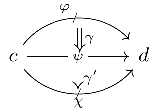
You can remember the direction \varphi\Rightarrow\psi because in the parallel arrows \varphi\mathbin{\triangleleft}\gamma and \gamma\mathbin{\triangleleft}\psi above, you can see that \varphi comes before \gamma and \psi comes after \gamma. But what does a map \gamma satisfying (1) mean?
Recall that a map \gamma\colon c\to\mathcal{y} is a global section (Aguiar calls it an admissible section). It assigns to each object I:c(1) an outfacing morphism \gamma^\sharp_I\colon I\to I', from I to some other object I'\coloneqq\mathop{\mathrm{cod}}\gamma^\sharp_I. The counit \epsilon\colon c\to\mathcal{y} is such a thing: it assigns to each I the identity on I, as an outfacing morphism. But in general, \gamma is like a vector field—or we could call it a direction field—on your category: wherever you are, this is the direction \gamma is telling you to go. Let’s denote the set of direction fields on c by \Gamma_c\coloneqq\mathbf{Poly}(c,\mathcal{y}).
So the data of a natural transformation between cofunctors out of c is just a direction field \gamma\in\Gamma_c. Untangling the commutative diagram (1) is a matter of careful element-tracking, and I find it to be most easily done using polyboxes. Allow me to unpack it for you.
Given any object I:c(1), define I'\coloneqq\mathop{\mathrm{cod}}(\gamma^\sharp_I) and J\coloneqq\varphi_1(I). So we have a map \gamma^\sharp_I\colon I\to I' in c and an object J:d(1). Finally, let g:d[J] be any map out of J. The commutativity of (1) says two things:
there is an equality of objects J=\psi_1(I')
letting f\coloneqq\varphi^\sharp_I(g) and f'\coloneqq\psi^\sharp_I(g), there is an equality of morphisms f\mathbin{;}\gamma^\sharp_{\mathop{\mathrm{cod}}(f)}=\gamma^\sharp_I\mathbin{;}f'
Here’s a picture, with top layer in c and bottom layer in d, with \varphi maps drawn blue rightward and \psi maps drawn red leftward, and with the natural transformation data \gamma shown as dashed.
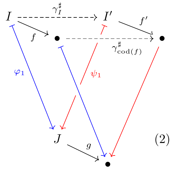
For every object I in c we get such a dashed map I\to I' for some I', and for every morphism out of the mutual image downstairs, we get a commuting square upstairs.
It’s not hard to see the analogy with natural transformations between functors. For functors, the data is a morphism in d for every object in c; for cofunctors it is a morphism in c for every object in c. For functors, any morphism in c gives you a commuting square in d; for cofunctors you only need to pay attention to morphisms out of objects in the image of \varphi, but for any such morphism you get a commuting square in c. And just like how natural transformations between functors don’t really involve the identities or compositions on the domain side (other than for defining the functors), natural transformations between cofunctors don’t really use the identities or compositions on the codomain side (other than for defining the cofunctors).
By the way, discrete opfibrations can be regarded both as functors and as cofunctors, so it’s reasonable to wonder whether the two notions of natural transformation—between them as functors and as cofunctors—coincide. Brandon Shapiro and I convinced ourselves with a convoluted argument that they do coincide, except that the two notions point in opposite directions. I reached out to Bryce Clarke to confirm, and he responded with a very elegant proof that this is correct, so thanks to him for that! But because the two notions point in opposite directions in the best of cases and are even more deeply opposite in other cases, I feel a bit torn as to whether we should call the maps between cofunctors ‘cotransformations’ (following Aguiar) or ‘transformations’ (following Clarke and di Meglio). For this blog post, which is pretty low-stakes, I’ve decided it’s best to follow Clarke.
3 Vertical and horizontal composition
It’s pretty easy to guess what the identity natural transformation on some \varphi\colon c\nrightarrow d should be. We need a direction field \gamma\colon c\to\mathcal{y}, and we have \epsilon\colon c\to\mathcal{y} floating around. Trying it, we see that it works: the unitality of \epsilon and \delta imply that (1) commutes.
The vertical composition of natural transformations
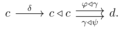
is slightly more surprising: given two polynomial maps \gamma,\gamma'\colon c\to\mathcal{y}, how should you “compose” them? It turns out that the set \Gamma_c of direction fields on a category carries the structure of a monoid. The idea is pretty easy: \gamma gives a morphism \gamma^\sharp_I\colon I\to I' out of any object I:c(1), and \gamma' gives a morphism \gamma'^\sharp_{I'}\colon I'\to I'' out of its codomain I':c(1), and you can simply compose them to get a morphism out of I. Mathematically, the “composite” of \gamma and \gamma' is given by the map c\xrightarrow{\delta}c\mathbin{\triangleleft}c\xrightarrow{\gamma\mathbin{\triangleleft}\gamma'}\mathcal{y}\mathbin{\triangleleft}\mathcal{y}\cong\mathcal{y}.
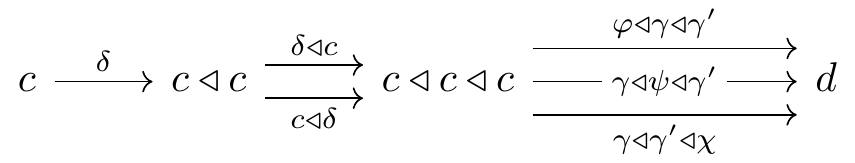
We have thus described a candidate for the composite \gamma\mathbin{;}\gamma', but does it make the diagram (1) commute? It’s pretty easy to visualize why it should, by looking at the diagram (2). And the formal proof is easy too: it involves this diagram:
Finally, suppose given natural transformations \gamma,\gamma' as follows:

note that \gamma gives rise to a unique polynomial map from c to c', namely \delta\mathbin{;}(\varphi\mathbin{\triangleleft}\gamma)=\delta\mathbin{;}(\gamma\mathbin{\triangleleft}\psi). Let’s call this \tilde{\gamma}\colon c\to c'. We can compose it with \gamma'\colon c'\to\mathcal{y} to get a map c\xrightarrow{\tilde{\gamma}\mathbin{;}\gamma'}\mathcal{y}, and this is the composite.
It’s often easier to think about whiskering than full-on horizontal composition. The whiskering of \varphi with \gamma' is simple: it’s just the composite direction field c\xrightarrow{\varphi}c'\xrightarrow{\gamma'}\mathcal{y}. The whiskering of \gamma with \varphi' is even simpler: it’s just \gamma!
4 Conclusion
Anyway, that’s it for now. I hope you agree that, once you know that the data of a natural transformation between cofunctors \varphi,\psi\colon c\nrightarrow d is just a map \gamma\colon c\to\mathcal{y} satisfying something..., you can kind of guess the rest, namely that it should make the two maps agree:
I find it striking that a single monoid, \Gamma_c, faithfully controls all the natural transformations between any two cofunctors out of c, as well as their identity and composition. That is, for any category d, there’s a faithful functor \mathbf{Cat}^\sharp(c,d)\to\Gamma_c to \Gamma_c as a one-object category. Have you ever seen anything like that?
Let me know your thoughts in the comments below!
Footnotes
In this post I’ll assume you know what a polynomial functor (in one variable, in \mathbf{Set}) is, my particular “positions and directions” vocabulary for it, and the notation (\varphi_1,\varphi^\sharp)\colon p\to q to refer to the “on-positions” and “on-directions” parts of a natural transformation, i.e. morphism of polynomial functors, \varphi\colon p\to q.↩︎