Lie groups induce Hopf monoids in Poly

Abstract

A Lie group G is a group object in the category of manifolds; that is, it’s a smooth space equipped with a special point e:G and a multiplication operation G\times G\to G. Every manifold M has a cotangent bundle T^*M\to M, and this can be made into a polynomial functor t^*_M. In this post we note what may be considered pretty obvious in retrospect: the polynomial t^*_G induced by the cotangent bundle on any Lie group G has the structure of a Hopf monoid.

Succinctly, a Hopf monoid is a bimonoid (i.e. it comes equipped with multiplication and comultiplication maps t^*_G\otimes t^*_G\to t^*_G and t^*_G\to t^*_G\otimes t^*_G, and unit and counit maps \mathcal{y}\to t^*_G and t^*_G\to\mathcal{y}, satisfying the usual equations) together with an antipode t^*_G\to t^*_G. The idea is to internalize the notion of a group in any monoidal category; in our case (\mathbf{Poly},\mathcal{y},\otimes).

I’ll explain the above in this post. In fact, we’ll see that the Hopf monoid leaves out a bit of the structure held by Lie groups, so we’ll append a bit more structure onto our Hopf monoids to capture it. Finally, we’ll explain what all this has to do with dynamic organizations, such as those found in deep learning and prediction markets.

1 Introduction

In any monoidal category, it’s worth asking:

1. what are the monoids?
2. what are the comonoids?
3. what are the frobenius monoids?

These can often have exciting answers, like “comonoids in (\mathbf{Poly},\mathcal{y},\mathbin{\triangleleft}) are exactly categories!”. When your monoidal category is symmetric, you can additionally ask:

1. what are the bimonoids?
2. what are the Hopf monoids?

This post is about Hopf monoids. Understanding bimonoids is 95% of the way to understanding Hopf monoids, so I’ll concentrate on bimonoids for now.

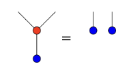
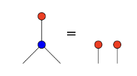
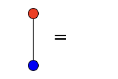
Bimonoids can be defined in any symmetric monoidal category, but I’ll use notation from (\mathbf{Poly},\mathcal{y},\otimes). A bimonoid consists of an object p, a unit and counit \mathcal{y}\xrightarrow{\eta} p \qquad\text{and}\qquad p\xrightarrow{\epsilon}\mathcal{y} and a multiplication and comultiplication p\otimes p\xrightarrow{\mu} p \qquad\text{and}\qquad p\xrightarrow{\delta} p\otimes p satisfying a bunch of rules. Namely, (p,\eta,\mu) is a monoid, (p,\epsilon,\delta) is a comonoid, and together they satisfy these four rules taken from nlab:

For a while, I could only think of a few bimonoids in \mathbf{Poly}. Namely, if (M,e,*) is any monoid in \mathbf{Set}, then M\mathcal{y} and \mathcal{y}^M are both bimonoids in \mathbf{Poly}. Indeed, both of the following functors are strong monoidal: (\mathbf{Set},1,\times)\xrightarrow{A\mapsto A\mathcal{y}}(\mathbf{Poly},\mathcal{y},\otimes) \qquad\text{and}\qquad (\mathbf{Set}^\textnormal{op},1,\times)\xrightarrow{A\mapsto\mathcal{y}^A}(\mathbf{Poly},\mathcal{y},\otimes) Hence, each sends monoids to monoids, comonoids to comonoids, and bimonoids to bimonoids. The downside is that neither M\mathcal{y} nor \mathcal{y}^M can be any more interesting than monoids are in \mathbf{Set}.

The purpose of this post is to explain why Lie groups—manifolds equipped with a group structure—provide a much more interesting source of bimonoids. In fact, they’re not just bimonoids, not just Hopf monoids, but even a little bit more: Hopf monoids equipped with a \mathcal{y}^\mathbb{R}-comodule structure. Let’s dive in.

2 Lie groups induce Hopf monoids in \mathbf{Poly}

The proof that Lie groups induce Hopf monoids in \mathbf{Poly} is very easy, once you know a few basic things.

Tangent space and cotangent spaces.

First recall the notion of tangent space for a manifold M. Given any point m:M, the tangent space, denoted T_mM, is the \mathbb{R}-vector space of all tangent vectors in M at m. The cotangent space, denoted T^*_mM is its vector space dual, i.e. it is the vector space of all linear maps T_mM\to \mathbb{R}. Given a map of manifolds f\colon M\to N, and any point m:M, we get a linear map T_m(f)\colon T_mM\to T_{f(m)}N forwards on tangent spaces; this is perhaps the most fundamental idea in differential geometry. From there it’s just a matter of composing linear maps to obtain a linear map T_m^*(f)\colon T^*_{f(m)}N\to T^*_mM\tag{\texttt{cotangent}} backwards on cotangent spaces.

To see how this all relates to polynomials, we begin with the cotangent bundle functor \begin{aligned} t^*_-\colon\mathbf{Mfd}&\to\mathbf{Poly}\\ M&\mapsto t^*_M\coloneqq\sum_{m:M}\mathcal{y}^{T^*_mM}\end{aligned} For any M:\mathbf{Mfd} we get a polynomial whose positions are the points of M and whose directions at m:M are the cotangent vectors (the “loss functions”) at m. To see that this assignment is functorial, we assume we’re given a map f\colon M\to N of manifolds, and we need a map on polynomials t^*_f\colon t^*_M\to t^*_N. Like any map of polynomials, it needs to go forwards on the positions and backwards on the directions. The map forwards on positions is just m\mapsto f(m), and for every position m:M the map backwards on directions is T_m^*(f) from (cotangent) above.

This functor is faithful, because given two different maps M\to N, they must differ on at least one point m:M, in which case we get two different maps t^*_M\to t^*_N. But more important for our purposes is the following.

The functor t^*_{-} is strong monoidal.

To say that t^*\colon(\mathbf{Mfd},\mathbb{R}^0,\times)\to(\mathbf{Poly},\mathcal{y},\otimes) is strong monoidal means that there is are isomorphisms t^*_M\otimes t^*_N\cong t^*_{M\times N} \qquad\text{and}\qquad \mathcal{y}\cong t^*_{\mathbb{R}^0} for any manifolds M,N. This comes down to the fact that for each m:M and n:N, we have T^*_{(m,n)}(M\times N)\cong T_m^*(M)\times T_n^*(N) \qquad\text{and}\qquad T^*_{\{\cdot\}}(\mathbb{R}^0)\cong 1.

Strong monoidal functors send monoids to monoids, comonoids to comonoids, bimonoids to bimonoids, and Hopf monoids to Hopf monoids. So our next task is to show that Lie groups are all of the above.

Lie groups are Hopf monoids in \mathbf{Mfd}.

You might think there’s a lot to check here—monoid structure, comonoid structure, interaction laws, etc—but in fact it all reduces quite a bit because we’re using the Cartesian structure (\mathbb{R}^0,\times) on \mathbf{Mfd}. In any Cartesian monoidal category, every object has the unique structure of a comonoid, and every monoid object has the unique structure of a bimonoid.

The fact that a Lie group G is a group object in (\mathbf{Mfd},\mathbb{R}^0,\times) is pretty much the standard definition. That is, we have a unit and a multiplication e\colon \mathbb{R}^0\to G \qquad\text{and}\qquad (*)\colon G\times G\to G satisfying the usual axioms. The comonoid structure is given by the unique map \epsilon\colon G\to\mathbb{R}^0 as the counit and the diagonal map \delta\colon G\to G\times G as the comultiplication.

Group structure.

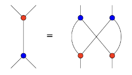
To say that a Lie group is a group, not just a mere monoid, we use the Hopf antipode map. This is a map \mathit{inv}\colon G\to G serving as the inverse. It makes both of the diagrams shown here commute: \tag{\texttt{antipode}} \begin{CD} G @>{\delta}>> G\times G \\@| @VV{G\times\mathrm{inv}}V \\G @. G\times G \\@V{\epsilon}VV @VV{(*)}V \\1 @>>{\eta}> G \end{CD} \qquad\qquad \begin{CD} G @>{\delta}>> G\times G \\@| @VV{\mathrm{inv}\times G}V \\G @. G\times G \\@V{\epsilon}VV @VV{(*)}V \\1 @>>{\eta}> G \end{CD} These say that for all g:G, writing g^{-1}\coloneqq \mathit{inv}(g), we have g*g^{-1}=1=g^{-1}*g.

And that’s it! Since Lie groups G are Hopf monoids in (\mathbf{Mfd},1\,\times) and since t^* is strong monoidal, we have that t^*_{G} is a Hopf monoid in (\mathbf{Poly},\mathcal{y},\otimes). Because \otimes is not the Cartesian structure in \mathbf{Poly}, the comonoid structure on t^*_G is nontrivial. In the next section we’ll explain what it captures about Lie groups and what it misses. Then we’ll add in the things that it misses.

3 What the Hopf monoid structure on t^*_{G} captures and misses

Nelson Niu and I wrote a paper a few years ago about what we called collectives. These are exactly the monoids in (\mathbf{Poly},\mathcal{y},\otimes), which in turn are exactly the lax monoidal polynomial functors.

So the math is that the condition of p being a \otimes-monoid, i.e. coming equipped with compatible maps \eta\colon\mathcal{y}\to p and \mu\colon p\otimes p\to p, is equivalent to the condition of the corresponding functor p\colon\mathbf{Set}\to\mathbf{Set} being lax monoidal 1\to p(1) \qquad\text{and}\qquad p(A)\times p(B)\to p(A\times B). For the intuition, Nelson and I explained that \otimes-monoids act like “compositional protocols for contributions and returns”. That is, think of any position P:p(1) as a contribution you can make, and for each contribution, think of the directions p[P] as what might possibly be returned to you, like “a return on your investment”. Then if a bunch of people each make a contribution, the \otimes-monoid structure provides a coherent way of combining them into one aggregate contribution, say P. It also provides, for any return r:p[P] to that aggregate contribution, a way of distributing r to each of the contributors, according to their specific contribution.

In the case of a Lie group G, we think of points g:G as contributions and covectors (or “loss functions”) \ell:T^*_g(G) as returns. Given a bunch (g_1,\ldots,g_n) of points, we can aggregate these contributions to obtain g\coloneqq g_1*\cdots*g_n. Then given any covector \ell:T^*_{g}G, we can break it up into n covectors, one at each of the contributing points g_i.

What is a \otimes-comonoid in \mathbf{Poly}? It turns out that these are exactly “collections of monoids”. That is, if we’re given compatible maps \epsilon\colon p\to\mathcal{y} \qquad\text{and}\qquad \delta\colon p\to p\otimes p then we can identify this with a set X\coloneqq p(1) for which each element x:X is equipped with a monoid M_x; its underlying set M_x\coloneqq p[x] is that of directions of p at x, its unit is given by \epsilon, and its multiplication is given by \delta.

In the case of a Lie group G, the fact that t^*_G is a comonoid says precisely that every cotangent space of G is itself a monoid: there’s a 0-cotangent vector and you can add cotangent vectors.

Now you might hope that the Hopf antipode map \mathit{inv}\colon G\to G, satisfying the diagrams in (antipode), would make each cotangent space a group, but it doesn’t! This information only tells us two things. First, that for any point g:G, there is an isomorphism \mathit{inv}_g^\sharp\colon T^*_gG\cong T^*_{g^{-1}}G between cotangent vectors at g and cotangent vectors at g^{-1}. And second, that we can take any cotangent vector \ell:T^*_eG at the identity and distribute it as a pair (\ell_1,\ell_2) of cotangent vectors \ell_1:T^*_gG and \ell_2:T^*_{g^{-1}}G such that 0=\ell_1+\mathit{inv}_g^\sharp(\ell_2). But without extra information, this doesn’t say that every cotangent vector in T_g^*G has an inverse; do you see a way we can get that from just the Hopf monoid structure on t^*_G? If so, please let me know in the comments!

I found the ability to enforce a group structure pretty sad at first. ¹ In fact, I realized that I was missing more than just negatives: I was missing the \mathbb{R}-module structure too. It turns out that we can get part of this—an \mathbb{R}-action—from additional structure on t^*_G. However, to get everything we want, e.g. inverses, we need to get down-and-dirty. Let’s begin with the nice part.

4 The \mathbb{R}-action on cotangent spaces

To get the next bit of structure, the \mathbb{R}-action, we need a little object called \mathcal{y}^\mathbb{R}. Since \mathbb{R} is a ring object in \mathbf{Set}, it is a co-ring object in \mathbf{Set}^\textnormal{op}, and so \mathcal{y}^\mathbb{R} is a co-ring object in (\mathbf{Poly},\mathcal{y},\otimes). That means that in addition to the completely uninteresting monoid structure !\colon \mathcal{y}\to\mathcal{y}^\mathbb{R} and \Delta\colon\mathcal{y}^\mathbb{R}\otimes\mathcal{y}^\mathbb{R}\to\mathcal{y}^\mathbb{R}, we have the following four maps (+), (*)\colon\mathcal{y}^\mathbb{R}\to\mathcal{y}^\mathbb{R}\otimes\mathcal{y}^\mathbb{R} \qquad\text{and}\qquad 0,1\colon \mathcal{y}^\mathbb{R}\to\mathcal{y} satisfying the comonoid axioms for (0,+) and for (1,*) as well as the distributive law with each other. Each of these comonoid structures also forms a bimonoid with the uninteresting (!,\Delta)-monoid structure. Finally, we have the Hopf antipode map \mathcal{y}^\mathbb{R}\to\mathcal{y}^\mathbb{R}, which serves as an additive inverse. We’ll be most interested in the (1,*)-comonoid structure.

A (\mathcal{y}^\mathbb{R},1,*)-coalgebra consists of a pair (p,\alpha), where p:\mathbf{Poly} and \alpha\colon p\to \mathcal{y}^\mathbb{R}\otimes p, satisfying the usual laws: \begin{CD} p @>{\alpha}>> \mathcal{y}^\mathbb{R}\otimes p \\@| @VV{1\otimes p}V \\p @= \mathcal{y}\otimes p \end{CD} \qquad\qquad \begin{CD} p @>{\alpha}>> \mathcal{y}^\mathbb{R}\otimes p \\@V{\alpha}VV @VV{(*)\otimes p}V \\\mathcal{y}^\mathbb{R}\otimes p @>>{\mathcal{y}^\mathbb{R}\otimes\alpha}> \mathcal{y}^\mathbb{R}\otimes\mathcal{y}^\mathbb{R}\otimes p \end{CD}

If p\coloneqq t^*M is the cotangent polynomial of a manifold, then the above coalgebra axioms say that for any point m:M and any cotangent vector w:T^*_mM, we have 1* w=w and r_1*(r_2* w)=(r_1*r_2)*w. Another axiom we can express is that the \mathbb{R}-action commutes with 0 and addition of cotangent vectors: r*0=0 \qquad\text{and}\qquad r*(w_1+w_2)=(r*w_1)+(r*w_2). These are encoded by the following diagrams: \begin{CD} p @>{\alpha}>> \mathcal{y}^\mathbb{R}\otimes p \\@V{\epsilon}VV @VV{\mathcal{y}^\mathbb{R}\otimes\epsilon}V \\\mathcal{y} @>>{!}> \mathcal{y}^\mathbb{R} \end{CD} \qquad\qquad \begin{CD} p @>{\alpha}>> \mathcal{y}^\mathbb{R}\otimes p @>{\mathcal{y}^\mathbb{R}\otimes\delta}>> \mathcal{y}^\mathbb{R}\otimes p\otimes p \\@V{\delta}VV @. @AA{\delta\otimes p\otimes p}A \\p\otimes p @>>{\alpha\otimes\alpha}> \mathcal{y}^\mathbb{R}\otimes p\otimes\mathcal{y}^\mathbb{R} @>>{\mathcal{y}^\mathbb{R}\otimes\sigma\otimes p}> \mathcal{y}^\mathbb{R}\otimes\mathcal{y}^\mathbb{R}\otimes p\otimes p \end{CD} Categorically, these axioms say that the \otimes-comonoid structure on p is compatible with the \mathcal{y}^\mathbb{R}-coaction. In other words, you can scale cotangent vectors by real numbers.

But to get the entire \mathbb{R}-module structure on these tangent spaces—in particular to know that (r_1+r_2)*w=(r_1*w)+(r_2*w), and in particular to get negatives, you need to go even further. This is the down-and-dirty part we referenced before.

The last step: using the monoidal fibration \mathbf{Poly}\to\mathbf{Set}.

The functor -(1)\colon\mathbf{Poly}\to\mathbf{Set} sends a polynomial p to its set of positions p(1), and this is a monoidal fibration in the sense of Shulman. ² It follows that we can identify this setup with a functor \mathbf{Set}^\textnormal{op}\to\mathbf{MonCat}. For each set P, we can consider the category \mathbf{Poly}_{P} of all polynomials whose set of positions is P; this is a monoidal category. The unit is P\mathcal{y} and the monoidal product for p_1,p_2:\mathbf{Poly}_{P} is given by p_1\otimes_P p_2= \sum_{a:P}\mathcal{y}^{p_1[a]}\otimes\sum_{a:P}\mathcal{y}^{p_2[a]}\coloneqq \sum_{a:P}\mathcal{y}^{p_1[a]\times p_2[a]} Let’s refer to this monoidal structure on \mathbf{Poly}_{P} as the P-local monoidal structure. One can check that it is cocartesian: P\mathcal{y} is the initial object and p_1\otimes_Pp_2 is a coproduct of p_1,p_2. In case it wasn’t clear, note that p_1(1)=P=p_2(1); we’ll continue that convention, and similarly also p(1)=P, below.

To finish off specifying the \mathbb{R}-module structure for p, we need to use this P-local monoidal structure on \mathbf{Poly}_{P}. Our comonoid maps \epsilon\colon p\to\mathcal{y} and \delta\colon p\to p\otimes p can be seen to factor through the P-local monoidal unit and product p\xrightarrow{\epsilon_{P}} P\mathcal{y}\to\mathcal{y} \qquad\text{and}\qquad p\xrightarrow{\delta_{P}} p\otimes_{P}p\to p\otimes p Every object in \mathbf{Poly}_{P} is uniquely a monoid (by virtue of (\mathbf{Poly}_{P},P\mathcal{y},\otimes_{P}) being cocartesian monoidal), and so if p is a comonoid in \mathbf{Poly} then it is a bimonoid in \mathbf{Poly}_{P}. Moreover, since the map \alpha\colon p\to\mathcal{y}^\mathbb{R}\otimes p is an isomorphism on positions, we can consider it as a map in \mathbf{Poly}_{P}.

So to get the \mathbb{R}-module structure on each commutative monoid of directions, we just ask for the following two diagrams in \mathbf{Poly}_{P} to commute: \begin{CD} p @>{\alpha}>> \mathcal{y}^\mathbb{R}\otimes p \\@V{\epsilon_p}VV @VV{0\otimes p}V \\P\mathcal{y} @>>{!}> p \end{CD} \qquad\qquad \begin{CD} p @>{\alpha}>> \mathcal{y}^\mathbb{R}\otimes p @>{(+)\otimes p}>> \mathcal{y}^\mathbb{R}\otimes\mathcal{y}^\mathbb{R}\otimes p \\@V{\delta_P}VV @. @AAA \\p\otimes_P p @>>{\alpha\otimes_P\alpha}> (\mathcal{y}^\mathbb{R}\otimes p)\otimes_P(\mathcal{y}^\mathbb{R}\otimes p) @= \mathcal{y}^\mathbb{R}\otimes\mathcal{y}^\mathbb{R}\otimes(p\otimes_P p) \end{CD} All combined, we now have that for each position a:p(1)=P, the direction set p[a] is an \mathbb{R}-module. The additive inverses we’ve been waiting for are simply defined as multiplication by -1:\mathbb{R}.

This last step, the one that relies on the monoidal fibration, is not as seamlessly part of what I call “the polynomial ecosystem”, because it’s not just about interactions between \otimes-bimonoids in \mathbf{Poly}. Instead it breaks the abstraction barrier and “escapes” into the underlying nuts and bolts of polynomial functors. It would be nice if somehow we didn’t need to do this, but currently I don’t see a way to avoid it.

5 Lie groups in dynamic organizations

Ok, so what can we use this for?

There is a monoidal bicategory called \mathbf{Org} that is useful for thinking about dynamic organizations: organizations of parts in wholes, where the organizational structure changes based on what flows. This structure, first defined here, underlies artificial neural networks and prediction markets, and it can also be found in Hebbian learning, and noncooperative games.

The objects of \mathbf{Org} are polynomial functors, \mathop{\mathrm{Ob}}(\mathbf{Org})=\mathop{\mathrm{Ob}}(\mathbf{Poly}) and the category of morphisms from p to q is [p,q]\textnormal{-}\mathbf{Coalg}. Often we’re interested in this when p\coloneqq p_1\otimes\cdots\otimes p_k and q\coloneqq q_1\otimes\cdots\otimes q_\ell. The idea is that the polynomials p_i,q_j are interfaces; we think of the p_i’s as more concrete and the q_j’s as more abstract. Morphisms \varphi\colon p\to q propagate data forwards as higher abstractions and also propagate feedback about those abstractions backwards. So let’s refer to such a morphism \varphi as an organization. Then [p,q]-coalgebras, i.e. morphisms in \mathbf{Org}, can be thought of as organizations whose forward and backward maps change based on what exactly is sent forward and backward through them. Let’s call these coalgebras dynamic organizations. Ones that don’t change—they just stay at some \varphi forever—could be called static organizations.

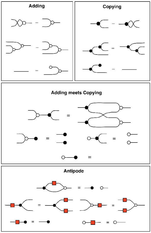
What monoids, comonoids, bimonoids, and Hopf monoids do in this context is that they give rise to static organizations which we can use to convert between different kinds of dynamic organizations. That is, if q is a comonoid, we can turn [q\otimes q,r]-coalgebras into [q,r]-coalgebras and [p,q]-coalgebras into [p,q\otimes q]-coalgebras. If q is a monoid, we can turn [p,q\otimes q]-coalgebras into [p,q] coalgebras and [q,r]-coalgebras into [q\otimes q,r]-coalgebras. So if q is a bimonoid, e.g. if q=t^*_G for some Lie group G, we can do all combinations of these, and more. In particular, we get a kind of graphical linear algebra string diagram syntax, as in Pawel Sobocinski’s blog.

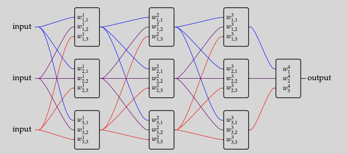
For example, in deep learning, it is quite common to use the comonoid operation to “split the axon” coming out of any box

6 Conclusion

Hopf monoids in \mathbf{Poly} are interesting in the context of dynamic organizations, because they allow us to statically merge and duplicate objects. So far, the only Hopf monoids I know of are the linear and representable polynomials G\mathcal{y} and \mathcal{y}^G on any group G, and the cotangent bundle t^*_G of any Lie group G, as well as tensor products of the above. If you can think of another one, please leave it as a comment below!

As for Frobenius monoids in \mathbf{Poly}, I feel like I knew at one point that they were very “boring”, but I’ve forgotten the proof now. Please also let me know in the comments if you have thoughts about them.

Footnotes

1. I get a bit emotional when mathy things don’t work like I expect. When I was about 5 years old, I suddenly realized the most amazing thing. If you write with pencil on an eraser, the mark will disappear instantly! I didn’t know how, but I knew it would work somehow, and I couldn’t wait to see it in action. How would it look while it was happening??! I finally got back to my desk from wherever I was; I took out my pink eraser and my pencil, and I wrote a line on the pink eraser. The line just stayed there, and I just stared at it in disbelief. How could this not work?!! And so it felt some forty years later with Lie groups as Hopf monoids in \mathbf{Poly}: the inverse was not as cool as I was expecting it to be.

2. That is, the functor -(1)\colon\mathbf{Poly}\to\mathbf{Set} is a fibration that extends to a strict monoidal functor (\mathbf{Poly},\mathcal{y},\otimes)\to(\mathbf{Set},1,\times), the codomain is Cartesian monoidal, and \otimes preserves cartesian arrows.