Poly inside Poly

Abstract

In this post, I’ll explain how to use Steve Awodey’s notion of universe to represent the set of polynomials as a certain naturally-derived object in Poly: “Poly inside Poly”. That is, given a universe u there’s an associated polynomial functor w that encodes u-small polynomials, and also encodes the closure of u-small polynomials under dependent sums and products, and under various other operations.

Edit, 2022-02-03: This post references a previous blog post, which I have since realized contains a crucial error: the claimed self-distributive law on the free monoid monad does not exist. As a result, what I call w=u\triangleleft u does not seem to have a monad structure after all. It somehow “should”—the intuition below is tantalizingly close to correct—but it runs into the 1-dimensionality of the category \mathbf{Poly}, which I’m sure my HoTT friends saw coming. Anyway, I apologize for the error. If you’re still interested in reading, please take everything below with plenty of salt.

1 Introduction

In March, Steve Awodey gave a talk at the Polynomial Functors workshop about how a universe type is a polynomial monad u with extra structure. I was quite intrigued and noticed that he was somehow telling us about a distributive law \aleph\colon u\triangleleft u\to u\triangleleft u; I wrote a blog post about it here. Now it’s a bit embarrassing, but for some reason I didn’t at that point ask myself the question, “so how can we think about the monad structure on u\triangleleft u that arises from this distributive law?”

It turns out to be a fascinating story that somehow puts a decategorified version of \mathbf{Poly} inside of itself. That is, if we write w\coloneqq u\triangleleft u (double-u) to denote the carrier of this new monad then, as I’ll explain, w is a polynomial that itself signifies all the polynomials that can be formed within the universe u. For example, the list monad u=\mathit{list}=\sum_{N\in\mathbb{N}}y^N satisfies the axioms of a universe object, which we can think of as classifying finite sets; in this case w(1)=\mathit{list}(\mathit{list}(1))\cong\mathit{list}(\mathbb{N}) will be all lists of naturals, and a list of naturals (e.g. [1,4,3,0,3]) can be used to represent a polynomial (e.g. y+y^4+y^3+1+y^3). We see immediately that a position of w contains a bit more information than a polynomial (i.e. reordering the list to [4,3,3,1,0] does not change the polynomial, at least up to isomorphism), but for many intents and purposes we can think of w(1) as classifying u-ish polynomials.

In this post, I’ll explain these ideas, as well as operations on w that internally represent various monoidal and closure structures on \mathbf{Poly}, namely +,\times,\otimes, [-,-], \triangleleft. For each of these opearations on \mathbf{Poly}, I’ll give a corresponding operation on w, though somewhat surprisingly the operations for +,\times are maps w\times w\to w, whereas the operations for \otimes, [-,-], \triangleleft are maps w\otimes w\to w. I’m not exactly sure what to make of this, but the math is what it is. Let’s get to it!

2 Background: universe as monad with self-distributivity

I’ll start by reviewing the previous blog post. The idea is that a universe is a polynomial functor u that acts like “the set of cardinalities” of some maximal size. A great example to keep in mind is the “list” polynomial u:=\sum_{N\in\mathbb{N}}\mathcal{y}^N This would correspond to the universe of finite cardinalities: each position N\in u(1) is the name of a certain finite set of cardinality N, and its directions are the actual elements u[N]:=\{1,2,\ldots,N\} in that set.

The list polynomial is just an example, but a paradigmatic one. Our first job is to characterize what makes it good—what makes it universe-y. Awodey says that to ensure that it is sufficiently universe-like, we first want u to have dependent sums. That is, given a finite set N of finite sets M_1,\ldots,M_N, we want to be able to add them up and get a single set \sum_{i\in N}M_i. Moreover, each of its elements should correspond to exactly one element in exactly one of the M_i’s, and we want to know which one. All this is achieved with a cartesian monad structure on u, i.e. with two maps of polynomials \mathbb{1}:\mathcal{y}\to u\qquad\text{and}\qquad \Sigma:u\triangleleft u\to u that are iso on directions and that satisfy the monad laws. The unit map \mathbb{1} tells us which position in u corresponds to the unit type (the cardinality 1), and the map \Sigma tells us how to add up a list of cardinalities to get a cardinality. The monad laws say that adding up a 43-many cardinality-1 sets, or adding up just one cardinality-43 set, both yield 43, and also that this sort of set addition is associative.

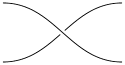
The other thing Awodey says we need to ensure that u is sufficiently universe-like is to give it dependent products. He did this one way (see his talk), but in my previous blog post I discussed a different way: namely, as a distributivity of the monad u over itself. Let’s draw distributivity u\triangleleft u\to u\triangleleft u this way, with one wire jumping over the other:

For notation, let’s denote the distributive law with an \aleph since that symbol looks like one wire crossing another:

\aleph:u\triangleleft u\to u\triangleleft u.

Here are the four axioms of distributivity, which look like dots passing though crossings:

In fact, we asked a little more of the universe, namely that \aleph factors through \text{indep}:u\otimes u\to u\triangleleft u, i.e. \aleph=\text{indep}\circ\nabla where \nabla has type

\nabla: u\triangleleft u\to u\otimes u.

The details are in the previous blog post, but the point is that these structures encode the fact that the universe u has dependent products. More concretely, it says that given a cardinality N and N-many cardinalities (M_1,\ldots,M_N), we can form two cardinalities, the product M:=M_1\times\cdots\times M_N and just N itself. Indeed this is what \nabla does on positions: it sends (N,(M_1,\ldots,M_N)\mapsto ((M_1\times\cdots\times M_N),N). Note that these two sets M,N are independent now: N does not depend on the product M, and that’s what the factorization \aleph=\text{indep}\circ\nabla says. But this is just the story on positions; on directions \nabla says that for any pair of elements (m, i)\in M\times N, we get an element in our original set N, namely i\in N, and we get an element in M_i, namely m(i)\in M_i.

Finally, all these structures “work right” in the sense of the four distributive laws shown graphically above. The reader can check for themselves what these four axioms mean about the product of a list of cardinalities. To compare with my answers: if A\in\mathbb{N} is a cardinality and B_1,\ldots,B_A\in\mathbb{N} are A-many cardinalities, and similarly for C_{1,1},\ldots,C_{1,B_1},\ldots,C_{A,1},\ldots,C_{A,B_A} are more cardinalities, then very schematically we have:

\begin{aligned} 1^A &= 1, \\ A^1 &= A, \\ (BC)^A &= B^AC^A, \\ (C^B)^A &= C^{(AB)}. \end{aligned}

These look like facts about products and exponents, but the products are actually dependent sums and the exponents are actually dependent products. Slightly less schematically, they say:

\begin{aligned} \Pi(A,1) &= 1, \\ \Pi(1,A) &= A, \\ \Pi(A,\Sigma(B,C)) &= \Sigma(\Pi(A,B),\Pi(A,C)), \\ \Pi(A,\Pi(B,C)) &= \Pi(\Sigma(A,B),C). \end{aligned}

And written out completely they say the following about cardinalities for dependent types:

\begin{aligned} \Pi_{a\in A}1 &= 1, \\ \Pi_{x\in 1}A &= A, \\ \Pi_{a\in A}\Sigma_{b\in B_a} C_{a,b} &= \Sigma_{b\in\Pi_{a\in A}B_a}\Pi_{a\in A}C_{a, b(a)}, \\ \Pi_{a\in A}\Pi_{b\in B_a}C_{a,b} &= \Pi_{(a,b)\in\Sigma_{a\in A}B_a}C_{a,b}. \end{aligned}

Again, the 1,\Sigma come from the monad structure on u and the \Pi with these four laws come from the distributivity law \aleph\colon u\triangleleft u\to u\triangleleft u.

3 The monad w\coloneqq u\triangleleft u as “poly inside poly”

I don’t know if it’s because I was so excited, lazy, uncourageous, or what, but when I found the above characterization, I completely forgot to pursue the most obvious thing you do when you have a distributivity structure between monads: I forgot to consider the composite monad! Luckily, my thoughts eventually returned to the subject, and I asked myself the question of how to think of this new monad; let’s call it “double-u”: w:=u\triangleleft u. As you might guess by the title of this post, w is a polynomial that itself represents polynomials p (where p has the cardinality bounds on both positions and directions dictated by u). Let’s begin by understanding how a position in w represents a polynomial.

As above, let’s think of u as the \mathit{list} functor u=1+\mathcal{y}+\mathcal{y}^2+\cdots. Then a position p\in w=u\triangleleft u denotes a list of natural numbers, e.g. p=[4,2,2,1,0,1]. We think of each list position i as representing a position of the polynomial “i\in p(1)”, so this list represents a polynomial with 6 positions. We think of the number p[i] in the ith entry of the list as representing the exponent, so this list p would correspond to the polynomial \mathcal{y}^4+\mathcal{y}^2+\mathcal{y}^2+\mathcal{y}+1+\mathcal{y}. Now we should be clear that w does not understand the relationship between the lists [4,2,2,1,0,1] and [4,2,2,1,1,0], even though they represent isomorphic polynomials. But that won’t stand in our way going forward; maybe it can be corrected with the right “groupoid” meta-theory; that’s a question for someone else at this point. The point here is that positions in w represent polynomials, or more precisely in the case of u=\mathit{list}, a position of w can be identified with a polynomial p for which the position-set p(1) and each direction set p[i] are linearly ordered.

We now understand the positions of w when u=\mathit{list}, so let’s move on to the directions. If p\in w(1) is a position, corresponding to a list of naturals with length denoted p(1), what is its set w[p] of directions? A direction in the composite w=u\triangleleft u consists of two dependent pieces: a direction for the first u, namely a choice of list position i\in p(1) and, depending on that, a direction for the second u, namely a choice of direction d\in p[i]. So the directions at p is w[p]\cong \dot{p}(1) the total set of directions for p. For the above p=[4,2,2,1,0,1], a direction is an element between 1 and 10=4+2+2+1+0+1. In summary, a position of w corresponds to a polynomial and the direction-set there is the direction-set of that polynomial.

Back to a general universe u as above (no longer just list), we’re considering the monad structure \eta:\mathcal{y}\to w\qquad \mu\colon w\triangleleft w\to w on w as the one coming from the distributivity structure \aleph\colon u\triangleleft u\to u\triangleleft u. It turns out that this monad structure basically represents the fact that polynomials are closed under dependent sums and dependent products: we can take a sum of products of polynomials and get a polynomial.

When u=\mathit{list}, the unit of the monad u is the one-element list, so the unit of w picks out the identity polynomial, represented by the one-element list [1]. The multiplication map \mu\colon u\triangleleft u\triangleleft u\triangleleft u\to u\triangleleft u is more interesting: on positions, it takes a list of lists of lists of naturals and produces a list of naturals. Said another way, it takes a list of lists of polynomials and produces a polynomial. Given a list of lists of lists of naturals, think of the outer-most list as the list of summands, the next level list as the list of factors, and the remaining list of naturals as a polynomial (like we did above). So for example, the sum-of-products \big((\mathcal{y}+1)\times(\mathcal{y}+1)\big)+\big(\mathcal{y}\times(\mathcal{y}^3+\mathcal{y}+2+\mathcal{y})\times(\mathcal{y}^2+1)\big) would be represented as the list of lists of lists of naturals \Big[\big[[1,0],[1,0]\big],\big[[1],[3,1,0,0,1],[2,0]\big]\Big]. The job of \mu (on positions) is to evaluate that sum of products of polynomials to obtain a single polynomial, namely [2,1,1,0,6,4,4,2,4,2,3,1,3,1] In other words, the above sum of products evaluates to \mathcal{y}^6+3\mathcal{y}^4+2\mathcal{y}^3+3\mathcal{y}^2+4\mathcal{y}+1. And given a direction d in that resulting polynomial, the on-directions part of \mu finds “where it came from”, i.e. it picks out the unique summand and the unique factor polynomial and the unique direction in that polynomial which together gave rise to d. Pretty cool, huh?

Now we see that w represents the objects of \mathbf{Poly}, together with their closure under dependent sums and products. One of the things I’m most curious about is whether there’s a way to get the morphisms of \mathbf{Poly} inside of \mathbf{Poly} as well. I’m not sure how to explain this question other than the appeal “If w represents the objects of \mathbf{Poly}, where are the morphisms?” I fear that the difficulty I’m having here is well-known to people who think about universes a lot (or maybe even a little), and maybe there’s no use in trying to find it, but I’d be quite pleased to find something suitable. But for now, I want to tell you about how to encode the monoidal operations on \mathbf{Poly}, in terms of operations on w.

4 Four monoidal operations and a closure

First, polynomials are closed under binary sums and products, and correspondingly (at least if your universe u contains a notion of “2”) we can find maps \textnormal{"}+\textnormal{"}: w\times w\to w \qquad\text{and}\qquad \textnormal{"}\times\textnormal{"}: w\times w \to w that encode these. The “+”-map takes a position (p,q)\in (w\times w)(1) and returns a position corresponding to p+q. For example, if u=\mathit{list} then it would take [3,1] and [1,1,1] (corresponding to \mathcal{y}^3+\mathcal{y} and 3\mathcal{y}) and return [3,1,1,1,1] (corresponding to their sum). Moreover the “+” map is cartesian; i.e., there is a bijection w[p+q]=\dot{p}(1)+\dot{q}(1)\cong(w\times w)[(p,q)]. Similarly, the “\times”-map takes a position (p,q)\in (w\times w)(1) and returns the position p\times q, and on directions is given by w[p\times q]=q(1)\dot{p}(1)+p(1)\dot{q}(1)\to \dot{p}+\dot{q}(w\times w)[(p,q)].

But in fact, we can get n-ary addition and multiplication for free from the monad structure on w, and recover the above. Namely, we have two maps (\mathbb{1}\triangleleft u),(u\triangleleft\mathbb{1}): u\to u\triangleleft u=w. Thus we get two maps u\triangleleft w\rightrightarrows w\triangleleft w, and composing with the multiplication \mu:w\triangleleft w\to w, we get two maps u\triangleleft w\rightrightarrows w\triangleleft w\to w. When u=\mathit{list}, these two maps take a list of polynomials and respectively add them together or multiply them together. For example, they’d send [[1,0],[1,0],[0]] to [1,0,1,0,0] and [2,1,1,0] respectively, since (\mathcal{y}^1+\mathcal{y}^0)+(\mathcal{y}^1+\mathcal{y}^0)+(\mathcal{y}^0)=2\mathcal{y}^1+3\mathcal{y}^0 and (\mathcal{y}^1+\mathcal{y}^0)*(\mathcal{y}^1+\mathcal{y}^0)*(\mathcal{y}^0)=\mathcal{y}^2+2\mathcal{y}^1+\mathcal{y}^0.

If you want to recover the two descriptions above for adding or multiplying just two polynomials together, start with the cartesian map \mathcal{y}^2\to u, representing the cardinality “2”. Noting that \mathcal{y}^2\triangleleft w\cong w\times w, one can check that the two maps \mathcal{y}^2\triangleleft w\rightrightarrows w are the two maps “+” and “\times” described at the top of this section.

Somewhat surprisingly, the other operations we’ll discuss, namely “\otimes”, “\triangleleft”, and “[-,-]”, are all maps of the form w\otimes w\to w out of the tensor product w\otimes w rather than out of w\times w. I’m not sure how to think about that difference, but let’s ignore it and proceed. Basically, to get any of these three operations when u=\mathit{list}, you could just define by hand what it does on positions and I can just tell you that there will be an “obvious thing” to do with directions. Indeed, on positions, we need a map w(1)\times w(1)\to w(1), i.e. a way to take two polynomials (albeit with linearly ordered positions and directions) and spit out a polynomial; each of “\otimes”, “\triangleleft”, and “[-,-]” provides that information.

But I can do better than just assure you in the case u=list: I can tell you what these maps are for an arbitrary u. I’ll only write them out fully for “\otimes” and “\triangleleft”, because the case for [-,-] is messier. To define the w-version of “\otimes” we use the duoidality map (p_1\triangleleft p_2)\otimes (q_1\triangleleft q_2)\xrightarrow{\text{duoidal}}(p_1\otimes q_1)\triangleleft(p_2\otimes q_2) applied in the specific case that p_1=p_2=q_1=q_2:=u. We also use the lax monoidal functor \text{indep}:(\mathbf{Poly},\mathcal{y},\otimes)\to(\mathbf{Poly},\mathcal{y},\triangleleft) whose laxator is a natural map \text{indep}\colon p\otimes q\to p\triangleleft q, again in the specific case p=q:=u. And finally we use the monad structure \Sigma\colon u\triangleleft u\to u on the universe. Using these three maps, we can define “\otimes”: w\otimes w\to w to be given by the composite \begin{aligned} w\otimes w= (u\triangleleft u)&\otimes (u\triangleleft u) \\&\left\downarrow{\scriptsize\text{duoidal}}\right. \\(u\otimes u)&\triangleleft(u\otimes u) \\&\left\downarrow{\scriptsize\text{indep}\triangleleft\text{indep}}\right. \\(u\triangleleft u)&\triangleleft(u\triangleleft u) \\&\left\downarrow{\scriptsize\Sigma\triangleleft\Sigma}\right. \\u&\triangleleft u= w. \end{aligned} This just multiplies the positions and the directions, which indeed is the tensor product of polynomials.

To define the w-version of “\triangleleft”, we again use the laxator \text{indep}, applied in the specific case that p=q:=w. That is, “\otimes”: w\otimes w\to w is given by the composite w\otimes w\xrightarrow{\text{indep}} w\triangleleft w\xrightarrow{\mu} w. In other words, to compose polynomials (p,q)\in w(1)\times w(1), we think of p as denoting a certain dependent sum-of-products of polynomials, and then we apply this to just one polynomial, q, over and over. In other words we’re saying p\triangleleft q=\sum_{i\in p(1)}\prod_{d\in p[i]}q. The fact that q isn’t depending on i,d, even though it could have, is corresponding to the use of \text{indep} above.

The formula for “[-,-]” is more complex, but it too can be given as a composite of canonical maps including duoidality, swap (u\otimes u\to u\otimes u), \text{indep}, and the u and w monad multiplications \Sigma and \aleph. Basically, to construct it, you write out the formula for the internal hom [p,q] in \mathbf{Poly}, which uses only dependent sums and products [p,q]\cong\sum_{(j,d)\in\prod_{i\in p(1)}\sum_{j\in q(1)}\prod_{e\in q[j]}p[i]}\mathcal{y}^{\sum_{i\in p(1)}q[j i]} This is basically a recipe for how to use the monad and distributivity structures on u to form this internal hom as an operation on w.

5 Conclusion

To summarize, if we conceive of a universe of sets as a Cartesian polynomial monad (u,\mathbb{1},\Sigma), equipped with a self-distributivity structure \aleph\colon u\triangleleft u\to u\triangleleft u as I explained in a previous blog post, a natural question is to ask what the induced monad structure on w:=u\triangleleft u is. In the present post I showed that the carrier w can be interpreted as something like a decategorified version of \mathbf{Poly}, sitting inside of \mathbf{Poly}; the monad unit corresponds to the identity polynomial and the monad multipication corresponds to the closure of polynomials under arbitrary sums and products. I then showed how to reproduce four monoidal operations, +,\times,\otimes,\triangleleft, and a monoidal closure, [-,-], as various operations on w.

I’m not yet sure what to do with this. My hope was that somehow I could use w internally as a kind of programming language device. In fact Evan pointed me to this paper about the computer algebra system Maple which has (had?) a core data structure called the “sum-of-products representation” which is basically a list of lists of naturals (outer list is sum, inner lists are products, and numbers are exponents), just like in this post. Anyway, I had vague thoughts that having “poly inside poly” would give me something like Godel encodings or quines—that perhaps we could use w to let \mathbf{Poly} somehow “talk about itself”. So far, I haven’t found anything like that, at least beyond what’s written here, but maybe I will in the future. Or maybe you will! Please let me know if you have thoughts on this or similar topics.